2.9. Analysis of Results

---

download:pdf

---

2.9.1. Structure Optimization

2.9.1.1. Geometric Analysis

• General reports the symmetry information, such as space group, Pearson symbol and Wyckoff positions, as well as elementary physical properties such as cell volume and density

  

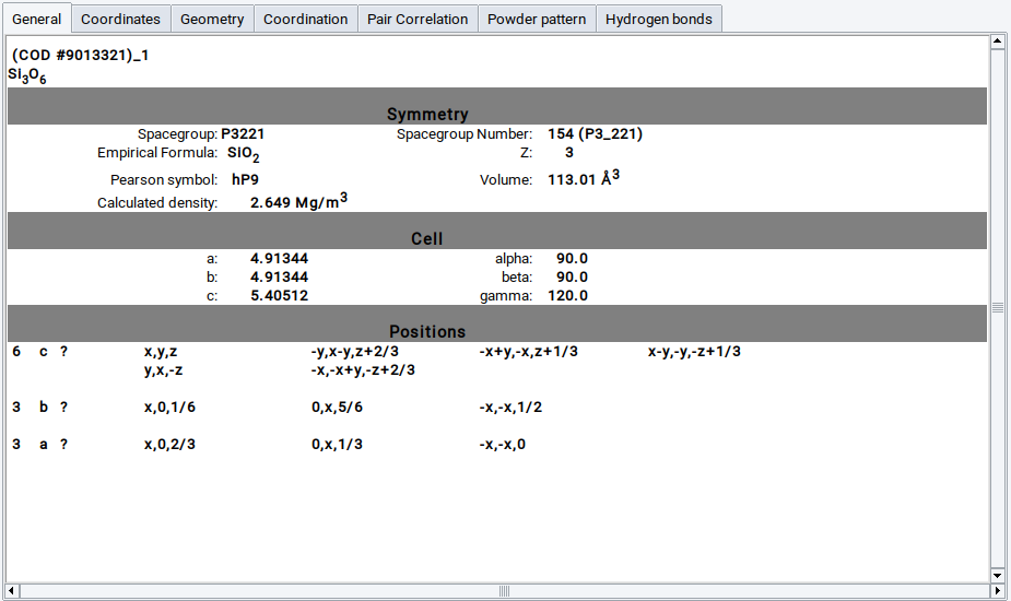
• Details about element positions are displayed in the Coordinates panel

• The Geometry panel prints distances and angles with neighboring atoms for a given reference atom

• In the Coordination panel, the number of nearest neighbors as a function of distance graph is plotted for a given reference atom

• The Pair Correlation panel graphically displays pair correlation functions for each element separately, as well as for the entire structure.

• Powder pattern shows the calculated [1] powder pattern for different X-ray sources (Co, Mo, Ag, Cr, Fe and synchrotron) and neutron scattering. The isotropic thermal coefficient (Biso) can be varied with the slider, the wavelength for synchrotron radiation and neutrons.

Experts use Copy lines as text to transfer the calculated angels and intensities to an external spreadsheet program.

2.9.1.2. (VASP) Trajectories, Trajectories, Gibbs Trajectories

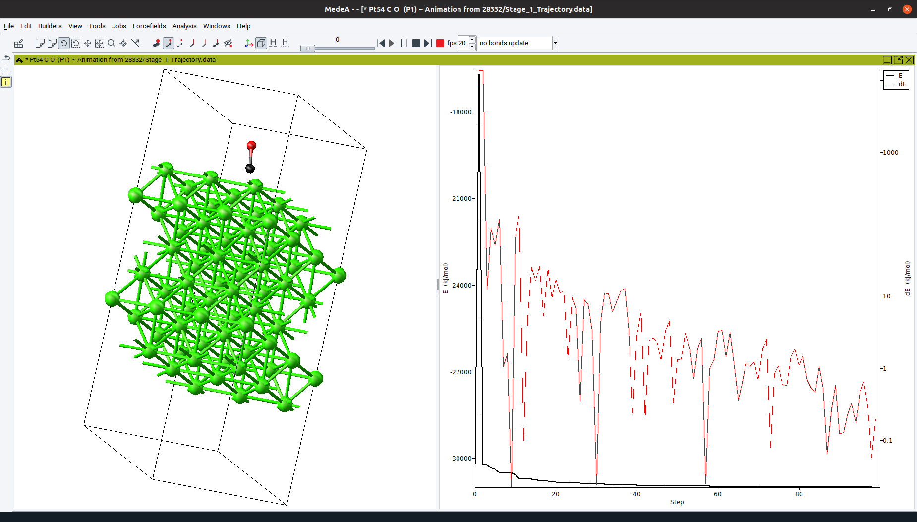
Trajectory opens a dialog listing all trajectory files of completed structure optimization and molecular dynamics runs. Select one or more structures to display a trajectory of their atomic positions and lattice parameters during the simulation as a function of the simulation step. For each trajectory, additional controls appear at the top of MedeA:

• The slider 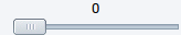on top allows moving to all intermediate frames between the initial (0) and final structures
• and skip to the initial and final structure, respectively
• Start the animation to cycle from the initial structure to the final structure and back with , pause it with
• Use to stop the animation and get back to the initial structure
• With the record button pushed, PNG files of each frame are saved while the trajectory is animated. The PNG files are written to subfolders in ~/MedeA/Movies, whereby “~” denotes the home directory of the MedeA user. The directory for movie creation is customizable via File >> Preferences…. The video can be created by concatenating the PNG files with an external program, such as ffmpeg located in MD/2.0/bin/Linux-x86_64 for Linux (or alternatively for your platform to be downloaded from https://ffmpeg.org/download.html) or the MovieMaker under Windows.
• The speed of the animation is controlled by the number of frames per second, set via the fps entry field or selector
• A pull-down menu allows you to select the way how bonds are updated during the trajectory animation. The default is to preform no bonds update, i.e. all bonds remain active independently where atoms are moving during the animation. Alternatively, bonds can be recalculated (created or removed depending on the geometry) for each geometry step, thus allowing for a dynamic adaption of bonds, either using the update bonds (distance + gap) algorithm or the update bonds (distance only) algorithm. These two bond algorithms correspond to the default mode to be customized from Bond Editor panel brought up from the Edit >> Edit bonds… menu item, and the alternative mode selected by checking the Use distance criterion only checkbox in the same panel, respectively.

In the right pane, for geometry optimizations the total energy (black curve) and the energy difference between two subsequent steps (red curve) are plotted for each geometry step (see Figure above). For molecular dynamics simulations, the total energy (black curve), kinetic energy (red curve) and potential energy (blue curve) are plotted as a function of the simulation time.

• Zoom-in on an area of interest by left-clicking in the graph and moving the mouse while holding the button
• Right-click to un-zoom or zoom back one level

Visualizing Gibbs trajectories of adsorption, only the gas phase molecules are displayed.

2.9.2. IR/Raman Spectra

Click on Analysis >> IR / Raman spectra to select results of calculations with computed IR and Raman spectra.

To compare with experimental data, you import spectra as csv file and display the calculated spectrum on top. Scale x-scale and intensity to match with experiment. Change the line width and, under more…., line shape (Gaussian or Lorentzian) until you are ready to Export… the spectrum.

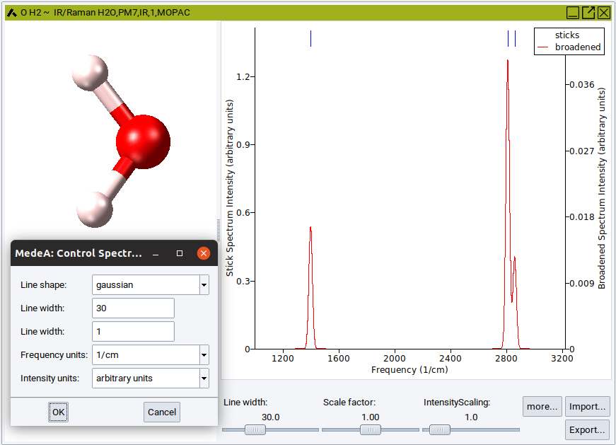
For spectra obtained from MOPAC the vibrational modes can be visualized by a right-click on the corresponding blue line above the peak and selecting Animate in the appearing pulldown menu. Animation of vibrational modes from Phonon calculations are not accessible directly from the IR and Raman spectra, but from the corresponding phonon dispersion curves. Handling, tuning and recording of animated vibrational modes are identical to those discussed in the previous section on trajectory animation.

2.9.3. Band Structure

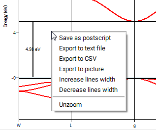
Click on Analysis >> Band Structures to open a dialog for selecting results from completed jobs. Selecting one or more jobs to open a graphics window showing the corresponding band structure plots. A BandStructure menu entry shows up in the menu bar, given access to further options.

• Uncheck As Lines to see all calculated points along the path, as shown on the right side

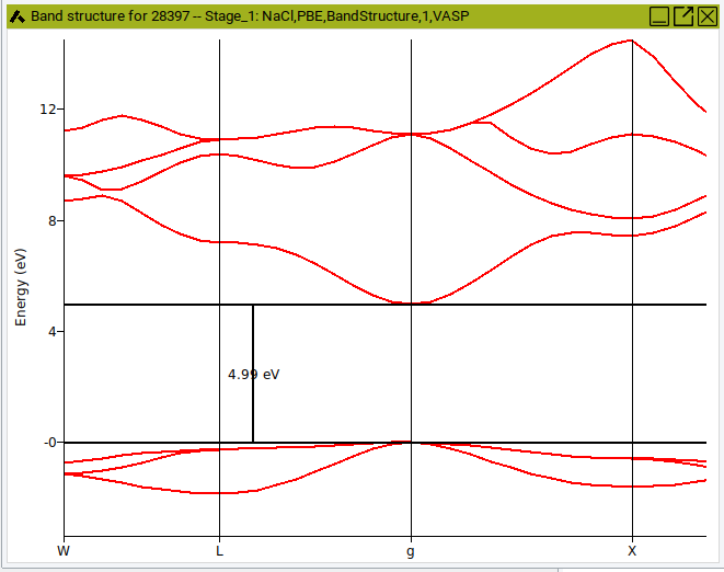
• Use Measuring lines to measure energy differences in the plot, you can move the lines by clicking on them and dragging them to a new position
• Left-click and hold to zoom into the plot
• Right-click and select Save as Postscript or Unzoom

2.9.4. Density of States

Click on Analysis >> Density of States to open a dialog for selecting results from completed jobs. Selecting one or more jobs to open a new window with the calculated density of states.

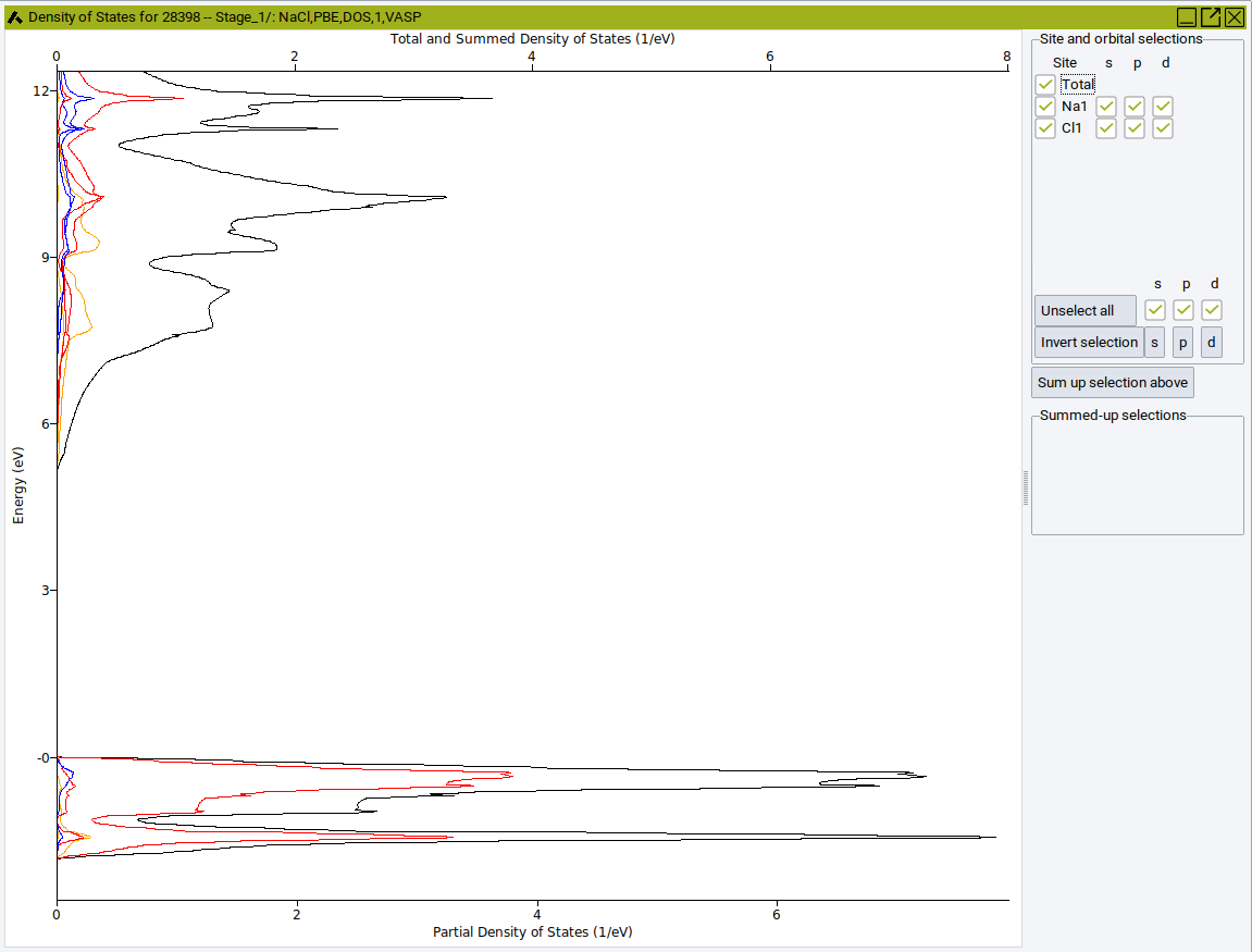
The color indicates the orbital or band: orange for s-states, red for p-states, blue for d-states and black for the total DOS.

• On the right-hand side, select a field to display or hide the corresponding partial DOS
• Click on an Atom label (e.g. Cl) to display or hide the contribution of the selected atom.
• Sum up selection combines selected atoms or orbitals.
• Moving the mouse over a line, highlights the corresponding atom of group (in this case Cl).

Please note different scale: total density of states at the top, partial density of states at the bottom.

Note

Core electrons are not included in the density of states. The attribution of electrons to specific atoms in solids is done by projecting the electronic density into spheres around the atoms. The corresponding sphere radii are arbitrary parameters, therefore the partial atomic density needs to be interpreted with care. In MedeA, covalent radii for each element are used as default values. To change the sphere radii, use the Add to Input section of the VASP interface(see The Vasp Guide for more details on the RWIGS keyword).

2.9.5. Optical Spectra

Click on Analysis >> Optical Spectra to open a dialog for selecting optical property results from completed VASP jobs. Selecting one or more jobs to open new windows with the calculated optical spectra as shown below.

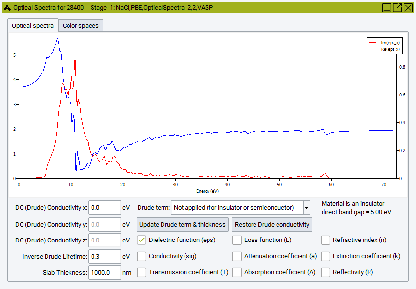
The optical spectra windows are initially created with the real and imaginary part of the dielectric functions, Im(eps) and Re(eps), plotted in the Optical Spectra Tab. In case of optically anisotropic materials, components in different Cartesian directions, such as Im(eps_x), Im(eps_y) and Im(epx_z) are displayed. There are a number of options to add and remove optical functions for display in the graph pane by means of the checkboxes at the bottom right of the Optical Spectra window:

• Dielectric function (eps): This toggles on and off the display of the real and imaginary part of the tensor elements of the dielectric function (epsilon). Individual components (depending on the symmetry of the system) can be displayed and hidden by selecting the legend fields to the right of the graph pane.
• Conductivity (sig): This toggles on and off the display of the real and imaginary part of the optical conductivity tensor elements (sigma) in units of eV, together with the legend entries Im(sig) and Re(sig) to the right of the graph, which can again be used to display or hide individual components.
• It is noted that dielectric function and conductivity tensor components refer to the scale to the left, which becomes highlighted in red color whenever the cursor touches one of these functions.
• Transmission coefficient (T): This toggles the display of the transmission coefficient (T) together with the legend entries for individual toggling. The transmission coefficient is strongly affetced by the Slab Thickness.
• Loss function (L): The loss function is the imaginary part of the inverse of the tensor of the dielectric function. This feature is not supported by MedeA 3.0.
• Attenuation coefficient (a): This toggles the display of the attenuation coefficient together with the legend entries for individual toggling.
• Absorption coefficient (A): This toggles the display of the absorption coefficient together with the legend entries for individual toggling.
• Refractive index (n): This toggles the display of the refractive index (n), i.e. the real part of the complex index of refraction, together with the legend entries for individual toggling.
• Extinction coefficient (k): This toggles the display of the extinction coefficient (k), i.e. the imaginary part of the complex index of refraction (sometimes denoted absorption index), together with the legend entries for individual toggling.
• Reflectivity: This toggles the display of the refractive index, together with the legend entries for individual toggling.
• It is noted that transmission, attenuation, absorption, and extiction coefficients as well as refractive index and Reflectivity refer to the scale to the right, which becomes highlighted in red color whenever the cursor touches one of these functions.
• Moving the mouse over a line highlights the line, the corresponding legend entry to the right and the scale to be applied for this function (either left or right). By means of the above checkboxes and legend entries any combination of optical functions can be displayed together in one graph.

The optical functions are processed differently, depeding on the existence of a band gap, i.e. depending on the metallic or insulating/semiconducting electronic structure of the system. The presence of a band gap is automatically detected by the underlying VASP calculation, and the information is provided beneath the graph on the right side, e.g. in the above example the Material is is an insulator with a direct band gap = 5.00 eV. For a metal it informs that the Material is a metal with no band gap. In case of metallic system the rather important intraband contribution is automatically added in an approximative manner by means of a Drude correction term mostly visible at relatively low frequencies. For insulating or semiconducting system the Drude term is not applied. Although the behavior at low frequencies is automatically adjusted to the detected system type, it can also be manually added or removed by the choice:

• Drude term: which directly adapts all optical functions according to the two possible settings

  • Applied (suitable for metal)
  • Not applied (for insulator or semiconductor)

The Drude term requires two parameters, the (in general direction dependent) Drude conductivity and the Drude lifetime. The Drude conductivity is automatically obtained from the plasma frequency as calculated by VASP, but can be modified from the entry fields

• DC (Drude) Conductivity x
• DC (Drude) Conductivity y
• DC (Drude) Conductivity z

The Drude lifetime is an empirical parameter and can be adjusted from the entry field

• Inverse Drude Lifetime: The default value is 0.3 eV.

Any changes to the settings for the Drude term, as well as a changes to the

• Slab Thickness in nm units

need to be applied by pushing the Apply Drude term & thickness button. In order to restore the default Drude conductivity values as derived from the plasma frequency values calculated from first principles, the button Restore Drude conductivity needs to be pushed.

There are several options to export the optical spectra to data files, all of which are accessible via a right-click on the graph pane. Like for all graphs, the picture can be exported to Postscript or tiff format, and the underlying data can be exported to text or CSV format. The context sensitive menu via right mouse click enables to increase or decrease line widths, and to change the energy/frequency/wavelength units.

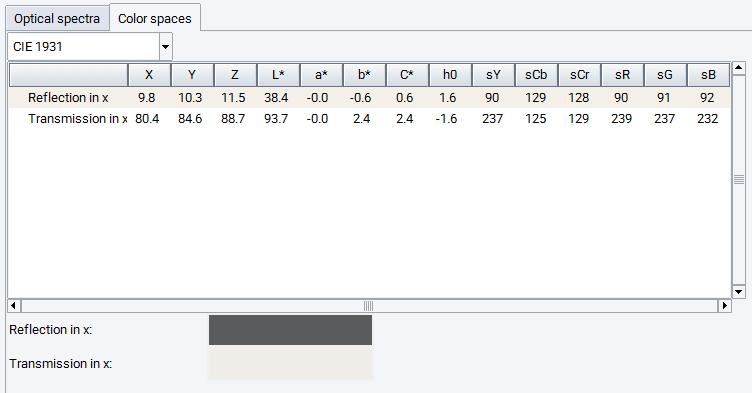
The second Tab of the optical spectra windows provides information on the Color spaces. Upon reflection and transmission (for optical anisotropic materials for different directions) a table provides the color space values of different conventions, based on the CIE 1931 or CIE 1964 standards, as well as the resulting RGB values. In addition, the RGB color values are shown by small canvas, demonstrating the predicted colors upon reflection and transmission (dependent on the Slab Thickness). For optical anisotropic materials color canvas for different Cartesian directions are shown.

2.9.6. Difference Charge Density

MedeA allows visualizing the pseudo charge densities and charge density differences. Charge density differences are defined as the difference between the initial, atomic charge density distribution as used by VASP to initiate a calculation and the final electronic charge density distribution as it results from a self-consistent calculation of the electronic ground state. The latter is very useful to observe where electrons move during the SCF cycle.

• To compute electronic charge densities and differences using VASP, (Pseudo, difference, spin) charge density in the Properties field of the VASP Calculation panel
• To visualize the difference in charge density, click on Analysis >> Difference Charge Density to open a dialog with a list of calculated charge densities. Select one or more structures to visualize their charge densities

The analysis window appears as a split structure window, the left-hand side showing the structure, the right-hand side showing four panels, IsoSurface (3D), Slice (2D), Averages (1D), and Points (0D). By default an isosurface with an average value of the difference charge density is shown.

In the IsoSurface (3D) tab you can:

• Specify the Iso value, using the slider or by typing in a value
• Choose a Color for the isosurface by clicking Choose color
• Type in a value to change the Transparency from invisible (0) to opaque (1)
• For quicker rotations and adjusting of the cell, the rendering quality can be modified by lowering the Precision from high to medium to very low
• Viewing Limits lets you display more than one unit cell of the structure. Click Update when making changes

Note

To improve the spatial resolution of the Difference Charge Density increase the values of the VASP parameters NGX, NGYF and NGZF. You find these values in the OUTCAR file, increase them, preferably to a power of 2. Use Add to Input in the VASP panel to add a line like NGXF=64; NGYF=64; NGZF=64 for increasing the computed default values.

In the Slice (2D) tab you can:

• Select planes by giving their Miller indices or a Normal unit vector
• Change the Altitude of a given plane by moving the slider or by typing in a value
• Use the color scale to change the color spectrum
• Change the range of values covered by the color spectrum using the small black arrows on the right
• Right-click into the color scheme and select Edit section to change the values and colors used as upper/lower boundaries. Click Apply to apply after making changes
• Right-click into the color scheme and select Add section above/below to add an additional section. For each section you can select a continuous spectrum of colors (ramp) or a constant value
• Edit as picture to get the current slice (without any superimposed cell boundaries and atoms), set the size to your specifications (either width or height) and save it as Bitmap, PNG or TIFF.

In the Averages (1D) tab you can:

• Select the axis normal to the averaged plane
• Integration range (in \({\mathring{\mathrm{A}}}\)) for the macroscopic averaging
• For further information push Help

In the Points (0D) tab you can:

• Add rows in a table with + and enter additional real space points in Fractional or Cartesian coordinates into the Table
• Calculate the values at these points by pushing Retrieve data
• For further information push Help

Example of Charge density difference for NaCl:

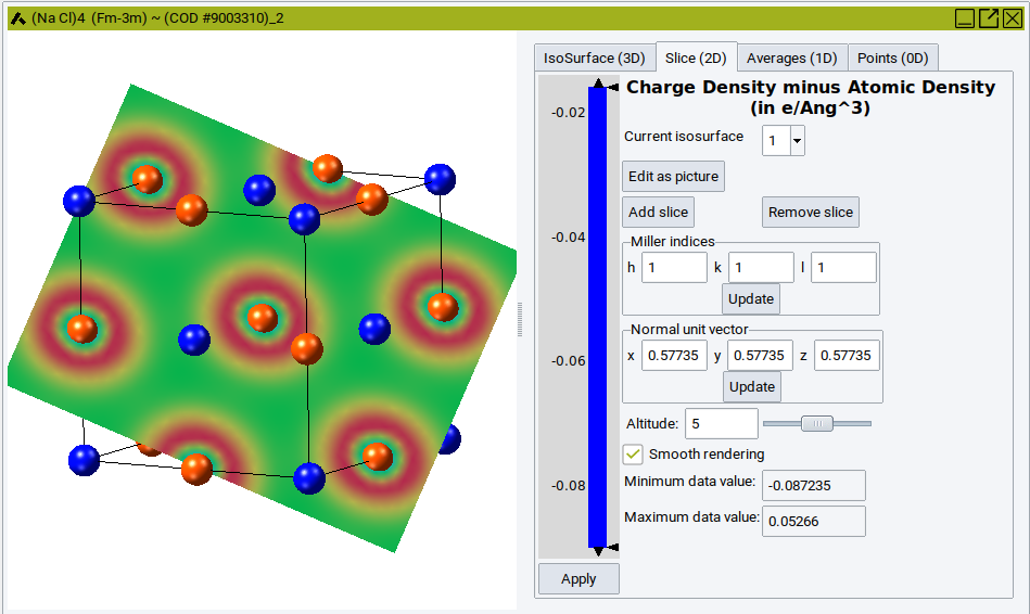
In the above example, a projection of the difference charge density onto the (111) plane is shown for NaCl. The range of the plot is from -0.087235 e\({\mathring{\mathrm{A}}}\)3 to 0.5266 e\({\mathring{\mathrm{A}}}\)3. The plot has three sections: The lowest section ranging from -0.09 to -0.016 is colored in blue. The section from -0.016 to 0.035 shows the variation of the difference charge density in colors from blue to red, the highest section is all in red. Depending on the altitude of the slice, not the full range of the variation in difference charge density is visible.

2.9.7. Magnetization Density

MedeA allows visualizing magnetization densities defined as difference between spin-up and spin-down electron density. To compute magnetization densities using VASP spin-polarized calculation, (Pseudo, difference, spin) charge density in the Properties field of the VASP Calculation panel

• To visualize a difference charge density, click on Analysis >> Magnetization Density to open a dialog with a list of calculated charge densities. Select one or more structures to visualize their magnetization densities.

The Analysis window has the same options as explained in the previous section.

It allows you to display

Note

To improve the spatial resolution of the Magnetization density increase the values of the VASP parameters NGXF,NGYF,NGZF.

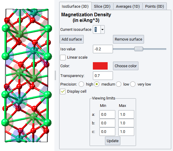
In the example above, the antiferromagnetic structure of Hematite (Fe2O3).

For structures with non-collinear magnetism, the analysis can be refined to x-, y- and z-direction.

In the Averages (1D) tab you can:

• Select the axis normal to the averaged plane
• Integration range (in \({\mathring{\mathrm{A}}}\)) for the macroscopic averaging

In the Points (0D) tab you can:

• Add rows in a table with + and enter additional real space points in Fractional or Cartesian coordinates into the Table
• Calculate the values of the magnetization density at these points by pushing Retrieve data
• For further information push Help

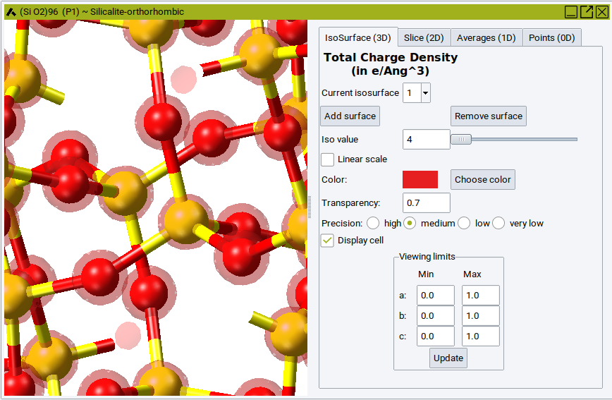
2.9.8. Total Charge Density and Total Valence Charge Density

MedeA allows visualizing total charge density and total valence charge densities. The total charge density includes all electrons including the core, the total valence charge density includes all electrons not included in the core of the pseudo potential or PAW potential.

• To compute these electronic charge densities using VASP, (Total, valence) charge density, Bader analysis in the Properties field of the VASP Calculation panel
• To visualize a valence charge density, click on Analysis >> Total Charge Density or Analysis >> Total Valence Charge Density to open a dialog with a list of calculated charge densities. Select one or more structures to visualize their charge densities.

The analysis window appears as a split structure window, the left-hand side showing the structure, the right-hand side showing four panels, IsoSurface (3D), Slice (2D), Averages (1D) and Points (0D). By default an isosurface with an average value of the total (valence) charge density is shown.

• Specify the Iso value, using the slider or by typing in a value
• Choose a Color for the isosurface by clicking Choose color
• Type in a value to change the Transparency from invisible (0) to opaque (1)
• For quicker rotations and adjusting of the cell, the rendering quality can be modified by lowering the Precision from high to medium to very low
• Viewing Limits lets you display more than one unit cell of the structure. Click Update when making changes

Note

To improve the spatial resolution of the Total Charge Density or Total Valence Charge density increase the values of the VASP parameters NGXF,NGYF,NGZF. You find these values in the OUTCAR file, increase them, preferably to a power of 2. Use Add to Input in the VASP panel to add a line like NGXF=64; NGYF=64; NGZF=64 for increasing the computed default values.

In the Slice (2D) tab you can:

• Select planes by giving their Miller indices or a Normal unit vector
• Change the Altitude of a given plane by moving the slider or by typing in a value
• Use the color scale to change the color spectrum
• Change the range of values covered by the color spectrum using the small black arrows on the right
• Right-click into the color scheme and select Edit section to change the values and colors used as upper/lower boundaries. Click Apply to apply after making changes
• Right-click into the color scheme and select Add section above/below to add an additional section. For each section you can select a continuous spectrum of colors (ramp) or a constant value.
• Edit as picture to get the current slice (without any superimposed cell boundaries and atoms), set the size to your specifications (either width or height) and save it as Bitmap, PNG or TIFF.

In the Averages (1D) tab you can:

• Select the axis normal to the averaged plane
• Integration range (in \({\mathring{\mathrm{A}}}\)) for the macroscopic averaging

In the Points (0D) tab you can:

• Add rows in a table with + and enter additional real space points in Fractional or Cartesian coordinates into the Table
• Calculate the values of the total (valence) charge density at these points by pushing Retrieve data
• For further information push Help

2.9.9. Pseudo Charge Density

MedeA allows visualizing pseudo charge densities used to construct the charge density differences. This includes all valence electrons not included in the core of the pseudo potential or PAW potential.

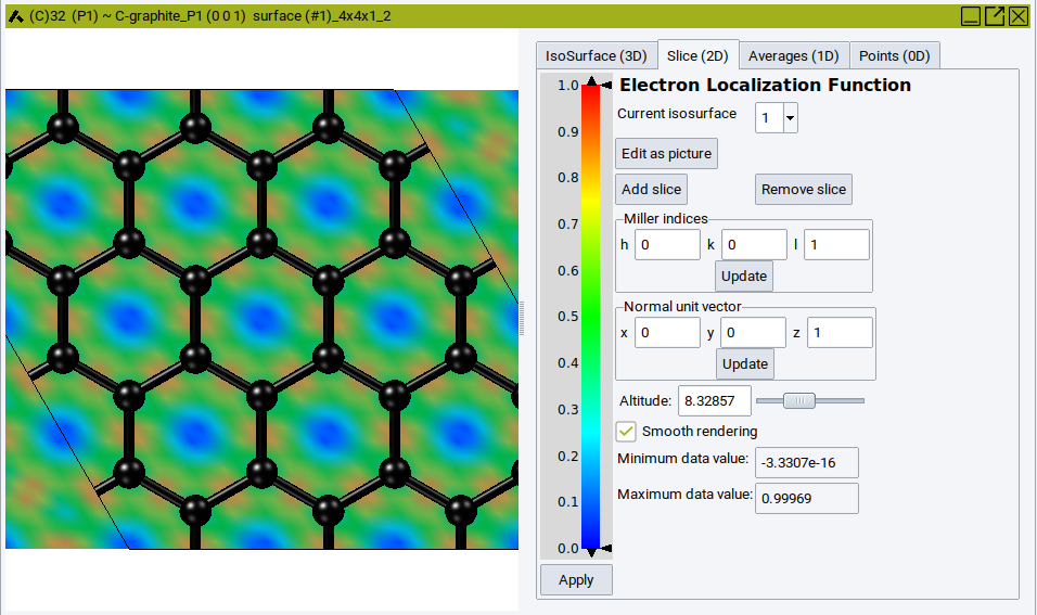
2.9.10. Electron Localization Function

The electron localization function [2], ELF, is used to identify binding and lone electron pairs in simple molecular systems. The MedeA interface for this feature is identical to the one for charge densities. The example below shows the a graphene plane.

Note

To improve the spatial resolution of the electron localization function increases the values of the VASP parameters NGX, NGY and NGZ. You find these values in the OUTCAR file, increase them, preferably to a power of 2. Use Add to Input in the VASP panel to add a line like NGX=64; NGY=64; NGZ=64 for increasing the computed default values.

2.9.11. Total Local Potential

The MedeA interface for this feature is identical to the one for charge densities and ELF.

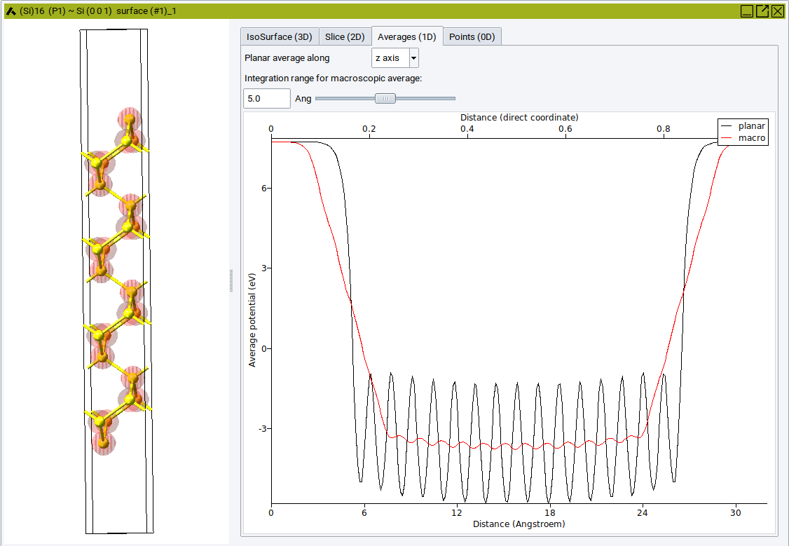
The Averages (1D) tab plots the total potential averaged over a plane normal to the selected axis.

Select an appropriate Integration range for macroscopic average to compare the total local potential between specific regions.

Note

To improve the spatial resolution of the local potential increase the values of the VASP parameters NGXF, NGYF and NGZF. You find these values in the OUTCAR file, increase them, preferably to a power of 2. Use Add to Input in the VASP panel to add a line like NGXF=64; NGYF=64; NGZF=64 for increasing the computed default values.

2.9.12. Export Band Structure and DOS

Sometimes it is very convenient to have the information from a calculated band structure or DOS calculation in numerical format and calculate band centers or highlight a specific band or surface modes for a publication.

First, select a list of jobs, which have band structure or DOS calculated. You might see a warning message reminding you that the VASP GUI allows for selecting band structure and DOS independently.

Some of the jobs that you selected do not have dispersion data. For these jobs, only the DOS data will be exported.

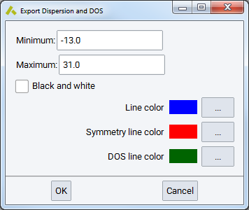
You can restrict the export to a narrower energy range, by setting a Minimum (eV) and Maximum (eV) on the scale relative to the Fermi energy (different from the values in the original VASP output files). These bounds are applied to the results of all selected jobs.

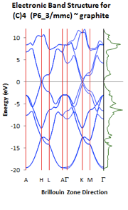
The color choices apply only to Excel and specify:

• Line color for bands
• vertical Symmetry line color and the
• color for the DOS line plotted on the right side of the band structure graph.

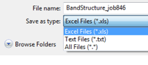
You can export the DOS values as a text file (.txt) or, if Excel is installed, also into a spreadsheet (.xls) which contains the band structure as well. The default format is an Excel file (.xls).

Please note, that you can also get the numerical data for a selected Band Structure or Density of States plot in MedeA by right-clicking into the active graphics panel and choosing one of the export options from the pulldown menu.

[1]	K Yvon, W Jeitschko, and E Parth\({\grave{o}}\) , “LAZY PULVERIX, a Computer Program, for Calculating X-Ray and Neutron Diffraction Powder Patterns,” Journal of Applied Crystallography 10, no. 1 (February 1, 1977): 73-74.

[2]	A D Becke and K E Edgecombe, “A Simple Measure of Electron Localization in Atomic and Molecular Systems,” Journal of Physical Chemistry 92, no. 9 (1990): 5397.

download:pdf