2.5. Special Builders
Contents
- Nanoparticles
- Nanotubes
- Nanowrap
- Nanowire
- Polymer Builder
- Defining Repeat Units
- Random Substitutions
- Amorphous Materials Builder
- Thermoset Builder
- Stack Layers Builder
- MedeA Docking
- Special Quasirandom Structures
- Build Surfaces
- Build Supercells
- Context Sensitive Menu for Molecular Structures
- Substitutional Search
- Merge
- Building Interfaces
- Conformers Search
- Structure List Editor
- Generic simple Forcefield (Minimization and Dynamics)
| download: | pdf |
|---|
2.5.1. Nanoparticles
Builders >> Nanoparticles… creates a spherical or cylindrical nanoparticle based on an existing periodic model and opens the molecular editor to fine tune the termination and set a cell size.
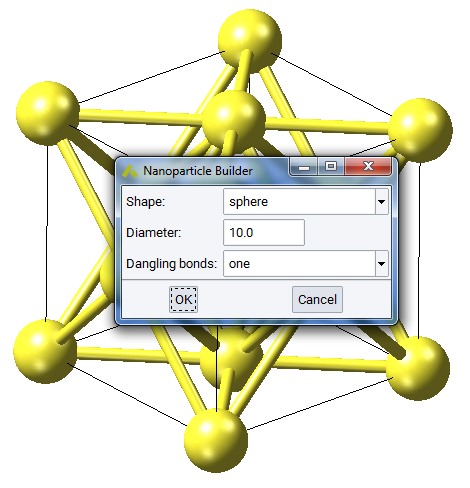
You need to specify the shape as sphere or cylinder, and set the size by diameter and length (for cylinder). Dangling bonds allows you to keep all existing bonds at the boundary, keep only one (for passivation) or none.
The initial nanoparticle is passed to the molecular editor (more details in II.D. 8. Edit in Molecular Builder), as you still have to decide on a cell size, in case you want to continue with a periodic model. You can passivate the dangling bonds with hydrogen, functional groups or with another element and continue passivating to build a bigger particle.
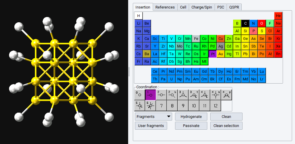
In the illustration below a spherical Au nanoparticle with 10 \({\mathring{\mathrm{A}}}\) diameter is passivated with Pt (with one-fold coordination).
2.5.2. Nanotubes
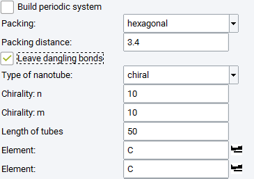
The Nanotube builder Builders >> Nanotubes… in MedeA creates periodic and isolated nanotubes from a flat sheet of graphene or related structure such as BN. You define basic requirements such as periodicity along the tube direction, packing in the perpendicular plane and the number of nested nanotubes. MedeA calculates the size of the resulting cell before building a system.
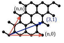
Type of nanotube: Nanotubes are defined by a chirality vector (n,m) which corresponds to how you fold a sheet of graphene into a tube. The two simplest nanotube orientations are armchair (n,n) and zigzag (n,0) and the corresponding chirality vector is shown in red.
Anything in between with 0<m<n is called chiral, for example the (3,1) direction is shown in blue. The Chirality vector m is set, but not editable, once you choose the zigzag or armchair type.
2.5.2.1. Periodic models
Check Build a periodic system to create infinitely long nanotubes of any type, otherwise you cut a nanotube of a defined length of tube.
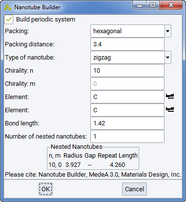
Packing: You can select hexagonal or cubic packing in the plane normal to the nanotube direction. The distance between nanotubes is defined by Packing distance (in Angstrom).
Number of nested nanotubes: With armchair and zig-zag orientation it, is easy to stack nanotubes of similar chirality, as they share the periodicity along the tube direction. For any other chirality MedeA requires that build periodic system is inactive. Otherwise the input field Chirality m is inactive and only zig-zag and armchair orientations can be chosen for nested nanotubes with periodicity.
2.5.2.2. Aperiodic models
You can still stack arbitrarily oriented nanotubes if you sacrifice the periodicity along the tube direction.
In this case you need to specify the Length of tubes (in Angstrom) and decide how to terminate the nanotubes.
Check Leave dangling bonds if you want to terminate with hydrogen.
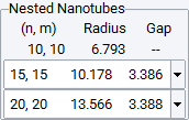
Nested nanotubes are defined by a spacing between walls and a tolerance of spacing.
The Nested Nanotube panel shows the defined sequence.
For non-periodic systems with fewer constraints, you can select any of the suitable nanotubes within the given Tolerance of spacing from the list.
You can easily create nanotubes of BN by changing the Element and Bond length.
2.5.2.3. Naming convention
CNT-(n,m). For periodic nanotubes, MedeA appends the label metallic or semiconductor to the name. Metallic nanotubes have (2n+m) or (n-m) divisible by 3.
2.5.3. Nanowrap
Build making use of Builders >> Nanowrap…. The Nanowrap surfaces into a cylindrical shape and works on periodic “surface” cells, where the vacuum of at least 4 \({\mathring{\mathrm{A}}}\) separates the top from the bottom.
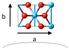
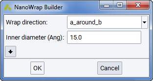
The top surface is going to be inside of a tube, the bottom surface outside. You have (at least) two choices to wrap a_around_b or b_around_a, Now click on OK.
Having VASP in mind, the default choice is to create the nanowrap with
the least number of atoms, so the suggested default is the shorter
vector b as the direction of the tube and wrap the longer vector a
as a  supercell around a circle, so that the inner
diameter (including the vacuum on top) is at least the requested 15 Ang.
supercell around a circle, so that the inner
diameter (including the vacuum on top) is at least the requested 15 Ang.
The shown Rutile 100 surface is red on top - and blue on the bottom and the grey circle indicates how we wrap the cell around.
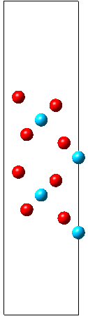
The lower layers are spread out considerably and to visualize bonds, you might need to set quite drastic values: Increase the minimum gap and the Bond cut-off factor by 2 or more. Obviously, the bond algorithm was not written for such weird and stretched bonds.
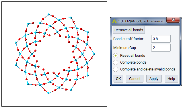
The bonds between atoms in the outer layers will be very stretched, so unless you protest we will stack the outer layers a little bit closer together.
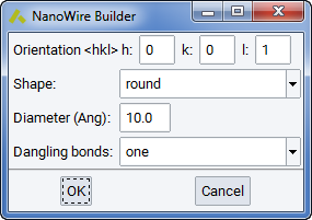
2.5.4. Nanowire
Nanowire building is accomplished by invoking Builders >> Nanowire… for a periodic bulk structure model. The control panel allows you to specify the wire’s Orientation <hkl> through the bulk crystal lattice, whether the Shape should be round, a square, or a rectangle, and allows you to enter the Diameter of the wire in units of Angstrom. The Dangling bonds choice allows you to keep all existing bonds at the boundary, keep only one (for passivation) or none. The resulting nanowire structure model is of molecular type, which can be transformed into a stack of wires by Create a periodic copy from the context menu (right-click into structure window) or by bringing up the molecular builder for this structure by hitting the corresponding icon in MedeA ‘s icon bar.
2.5.5. Polymer Builder
2.5.5.1. Features and Algorithm
The MedeA Polymer Builder constructs polymer models based on defined repeat units and rules concerning composition, orientation, and stereochemistry. A comprehensive collection of repeat units is supplied within MedeA, covering frequently encountered monomers, and repeat units may also be user defined, constructed in the Molecular Builder, and incorporated into polymeric systems using the Polymer Builder, allowing the construction of any desired polymer.
Polymers possess a great variety of possible microstructures. For example a simple polymer, based on a single repeat unit type, maybe isotactic, syndiotactic, or atactic.
| isotactic |  |
| syndiotactic | 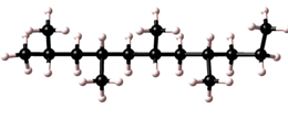 |
| atactic | 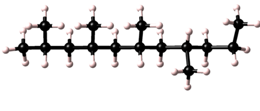 |
Polymerization may occur in either a head to tail, head to head (and tail to tail), or in a random sense.
| Head to tail | 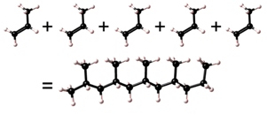 |
| Head to head | 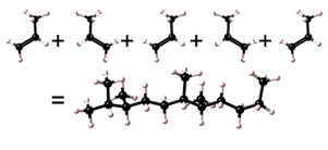 |
Additionally, the polymer backbone formed by the polymerization process possesses a conformation defined by a sequence of dihedral angles, and the ends of the chain may be terminated by capping groups or atoms (e.g. initiator and terminator fragments). Furthermore, when several repeat units are simultaneously polymerized, the composition of the polymer must be specified.
To accommodate these diverse building options intuitively, the Polymer Builder provides an interface, which progressively exposes options based on preceding selections. Hence, if a homopolymer (i.e. a polymer based on a single repeat unit) is to be constructed, options relating to copolymers are not presented in the user interface. Conversely, if multiple repeat units are specified, only options relating to copolymer formation are made available in the user interface, so that appropriate input may be provided. Hence the Polymer Builder allows complex polymers to be built with only the required options and settings presented to the user. Reasonable default options are provided whenever possible so that realistic polymer chains can be constructed straightforwardly.
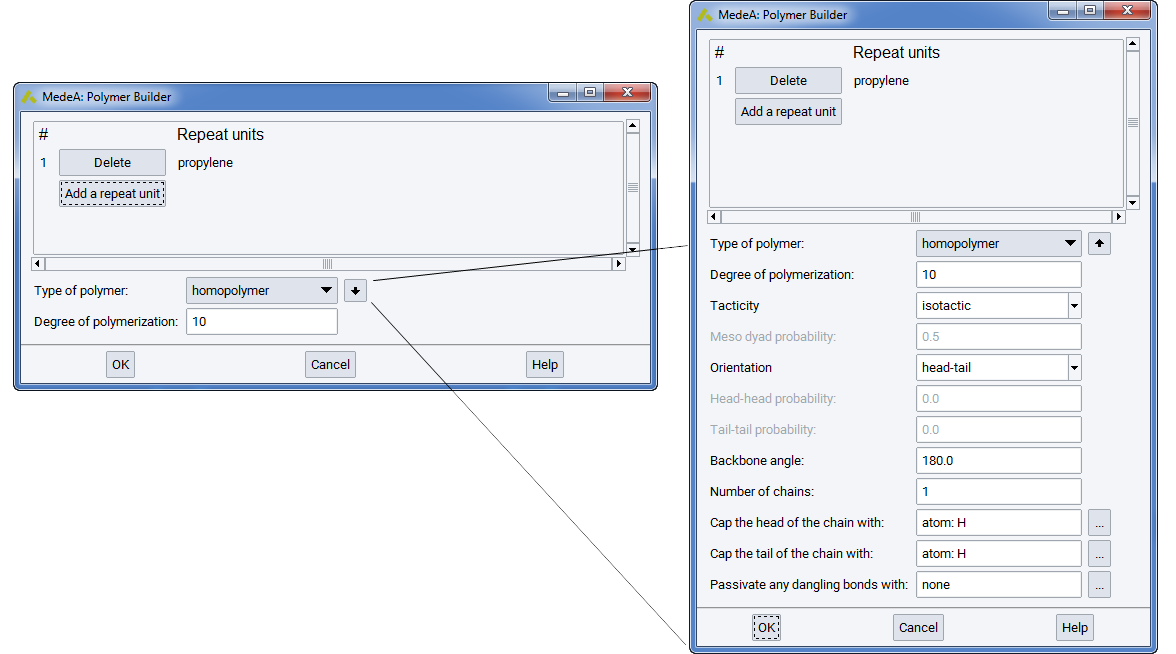
By default, the Polymer Builder presents the user interface shown in the figure below, which is invoked from the Polymers… menu item of the Builders menu of MedeA. This allows you to construct simply polymers and copolymers with minimal input information, making use of default settings. Additional input parameters may be selected through the ‘additional options’ button: \(\downarrow\). When the extended interface is selected, the ‘additional options’ button changes to \(\uparrow\), and clicking this arrow will remove the additional options from the Polymer Builder dialog box.
Algorithmically the Polymer Builder employs a construction process similar to that used by the Molecular Builder in combining molecular fragments, tuned for efficient construction of large polymers. At each stage in construction the fragment to be added to the growing polymer chain is translated and rotated to the required position, as defined by the existing backbone configuration and specified dihedral angle, and the appropriate bond created to add the repeat unit to the chain. This addition process is repeated for each repeat unit to match the specified input options.
When random copolymers are created the composition and stereochemistry of the polymer chain must be specified. This is accomplished through input parameters, which govern the fraction of each repeat unit expressed in the final polymer chain (which must sum to 1.0), and inversion and flip probabilities. The inversion probability describes the probability of pseudo chiral center inversion prior to polymerization, the flip probability describes the relative probability of head and tail connections occurring, for repeat units in which inversion of the connection direction causes differences in the resulting chain.
2.5.5.2. Usage
The steps required to create polymer models are as follows:
Select the required repeat unit, or units, from which the polymer is to be constructed
Select the type of polymer to be built; the options to choose between will depend on the number of repeat unit units selected. If a homopolymer (a single repeat unit) is selected, the required tacticity can be specified. If a copolymer (two or more repeat units) is selected, the appropriate copolymer type must be defined.
Select the degree of polymerization (the number of repeat units represented in the final polymer) or the block copolymer lengths.
Specify capping atoms, or fragments, and additional build options such as any required passivation of active bonds.
Construct the polymer, by clicking OK.
2.5.5.3. Default Parameters
In general the Polymer Builder provides reasonable default parameters. For example, polymer chains are passivated with hydrogen atoms, no additional active bond passivation is carried out, backbone dihedral angles are set to 180 degrees, and a single chain is constructed.
2.5.5.3.1. Parameters Common to all Polymers
Type of polymer
If just one repeat unit has been specified, the only available option is homopolymer.
If more than one repeat unit has been added to the repeat unit list, the options are:
alternating copolymer: e.g. ABABABAB…, ABCABCABC… etc.
block copolymer: e.g. AAAAAAABBBBBBB, AAAABBBBAAAA, AAABBBCCC etc. (where block sequence lengths must be specified in the repeat units’ list).
random copolymer: Completely random (‘statistical’) occurrence of repeat units, requiring specification of conditional probabilities for determining the probability pij that a repeat unit of type j attaches to a growing chain with repeat unit i at its end. See also section Parameters Specific to Copolymers for additional details)
Degree of polymerization - For a homopolymer or random copolymer, denotes the number of repeat units in the chain. For an alternating copolymer, denotes the number of times the alternating sequence is repeated. Note that for block copolymers, the number of repeats in each block is entered directly into the repeat unit window, and this entry field is not shown.
Backbone angle - Specifies the dihedral angle between successive repeat units. The convention is ‘180 degrees is trans’.
Number of chains - Number of independent polymer chains to build when the OK button is pressed.
Cap the head of the chain with: - Specifies the moiety to be attached to the beginning/head of the chain. Options are ‘H’, the name of a fragment, or ‘none’.
Cap the tail of the chain with: - Specifies the moiety to be attached to the end/tail of the chain. Options are ‘H’, the name of a fragment, or ‘none’.
Passivate any dangling bonds with: - When repeat units contain internal dangling/uncapped bonds, specifies the moiety to be attached. Options are ‘H’, the name of a fragment, or ‘none’.
2.5.5.3.2. Parameters Specific to Homopolymers
Tacticity - For vinyl and other repeat units containing pseudochiral centers (e.g. -CH 2CXY-), specifies the stereochemical configuration about the center. Options are isotactic, syndiotactic and atactic.
Meso dyad probability - For atactic chains, in which the stereochemical configuration is random, specifies the probability of two consecutive repeat units having the same chiral arrangement.
Orientation - Where appropriate (e.g. in vinyl polymers) specifies whether successive repeat units are connected in a head-to-tail, head-to-head/tail-to-tail or random pattern.
Head-Head Probability - Specifies the probability of attaching the next repeat unit via its head atom, when the atom at the end of a growing chain is also a head atom.
Tail-Tail probability - Specifies the probability of attaching the next repeat unit via its tail atom, when the atom at the end of a growing chain is also a tail atom.
2.5.5.3.3. Parameters Specific to Copolymers
Parameters are entered directly into the various fields displayed when the desired copolymer type has been selected. Required input for each copolymer type is:
Random (statistical) Copolymers
If the copolymer composition, as specified in MedeA’s File >> Preferences, is given in the form of:
Mole Fractions: Fraction - Denotes the mole fraction of the repeat unit listed in row i.
Conditional Probabilities: P1, P2, P3 etc - Specifies the conditional probability that the repeat unit in row i will be attached to a growing chain with repeat unit 1, 2, 3 etc. at its end. Values in each row must sum to 1.0.
Pinv - For repeat units containing pseudochiral centers (e.g. -CH 2CXY-), specifies the probability of inverting the stereochemical configuration about the center prior to adding the repeat unit to the growing chain.
Pflip - For situations in which repeat units can connect in head-to-tail or head-to-head arrangements (e.g.in vinyl polymers), specifies the probability of reversing the default head-to-tail mode of addition.
Block Copolymers
N - Indicates the number of repeat units of the type within each row/block.
2.5.5.3.4. Polymer Builder - Repeat Unit Dialog
The Repeat Unit dialog is displayed whenever the Add… button has been clicked in the Repeat units panel of the Polymer Builder dialog. Clicking on the selector button labeled Get the repeat unit from a allows repeat units to be obtained from one of three sources: repeat unit library, a Window in MedeA, or from a File. Now in more detail:
repeat unit library
Choosing this option displays a selection hierarchy with repeat units organized in folders according to common classifications, such as acrylics, amides, dienes, etc. Navigating to and selecting the desired repeat unit causes it to be displayed in the Repeat unit entry field. Clicking OK then closes the dialog and adds the repeat unit to the main dialog. Alternatively, double-clicking the repeat unit name closes the dialog and adds the repeat unit to the main dialog directly.
MedeA includes a large selection of common repeat units in its internal library. However, should it be desired to use a custom set of repeat units, these may be accessed by placing MedeA.sci files in a folder of the user’s choosing. The location of this folder is determined by the value of the User repeat unit library parameter in MedeA’s main File >> Preferences… dialog. The names of all .sci files in the user library folder are then displayed in a separate user folder appended to the repeat unit hierarchy dialog, and may be used in exactly the same manner as the repeat units provided with MedeA. Note that if the user’s repeat unit library does not exist, or is empty, this user folder will not appear in the display.
Note
Note also that user repeat units must contain valid repeat unit definitions for them to be included in the list.
window in MedeA: Choosing this option will inspect all current windows within MedeA for valid repeat units - defined as molecular fragments containing at least two ‘active’ bonds, one of which must have been designated as a ‘head’ atom, and the other as ‘tail’ (with only one head and tail permitted per repeat unit).
Any valid repeat units can then be chosen by using the Window selector button, followed by clicking OK.
file: This option allows the direct specification of a .sci file, without requiring that the repeat unit first be loaded into MedeA. Clicking the … button displays a traditional file browser enabling navigation to and selection of the .sci file containing the desired repeat unit definition.
2.5.6. Defining Repeat Units
As noted, the MedeA Polymer Builder constructs polymer models from defined repeat units. A comprehensive library of predefined repeat units is accessible from the Polymer Builder interface. Additionally, repeat units can be constructed using the MedeA Molecular Builder and saved in a user repeat unit library for later use.
To define a repeat unit in the Molecular Builder you construct a molecular fragment with active bonds at the desired head and tail connection points of the repeat unit. You then select the head and tail atoms and use the Define repeat unit command which is accessible from the right-click context menu of the Molecular Builder, under Selection, to identify the polymer backbone and connection points for the repeat unit.
The Define repeat unit command is accessible when two atoms are selected in the Molecular Builder. These selected atoms must also have active bonds. With standard graphics settings, repeat units are rendered in the MedeA Environment with green and red active bonds for head and tail atoms, respectively. Additionally, after the execution of the Define repeat unit command, backbone atoms in the repeat unit will be highlighted, so the structural characteristics of the newly defined repeat unit may be viewed and checked.
The initial selection of the head and tail atoms depends on the construction order of the molecular fragment, and if desired you may reverse the head and tail atoms with the Reverse repeat unit head and tail atoms command, which is also accessible from the Molecular Builder context menu, under the Selection command group.
Chiral and pseudochiral centers along the repeat unit backbone are identified by the Define repeat unit command, and this information is employed when the newly created repeat unit is used in the Polymer Builder to construct a polymer chain.
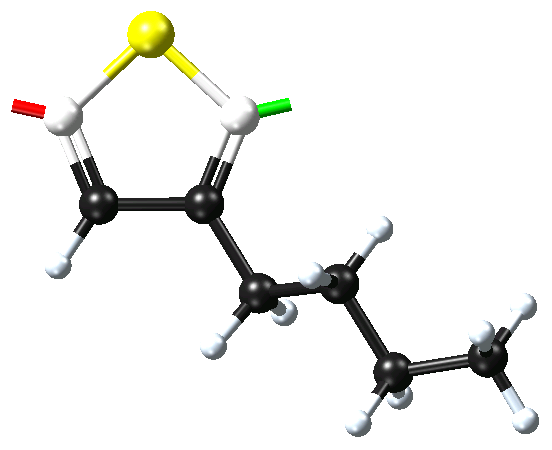
2.5.6.1. Constructing a Thiophene Polymer
To illustrate the use of the Polymer Builder and Define repeat unit commands we outline here the construction of a polythiophene derivative. Polymeric thiophene compounds possess interesting electronic properties including high conductivities when suitably doped, stimulating increasing technological interest. This example shows how polythiophene models with desired side chains can be constructed.
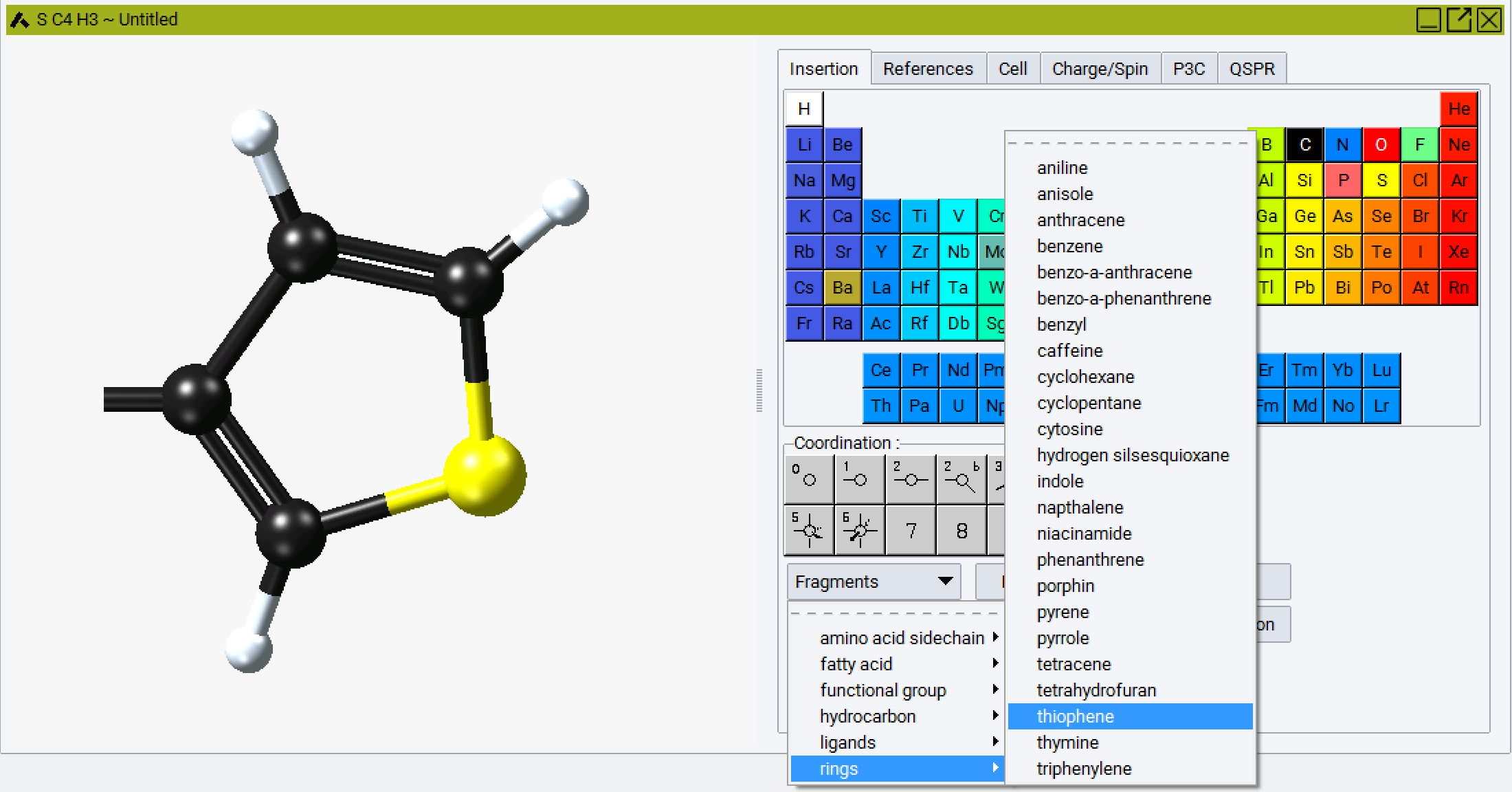
Begin by importing a thiophene fragment. This is best accomplished using the fragment library Molecular Builder and selecting a thiophene fragment:
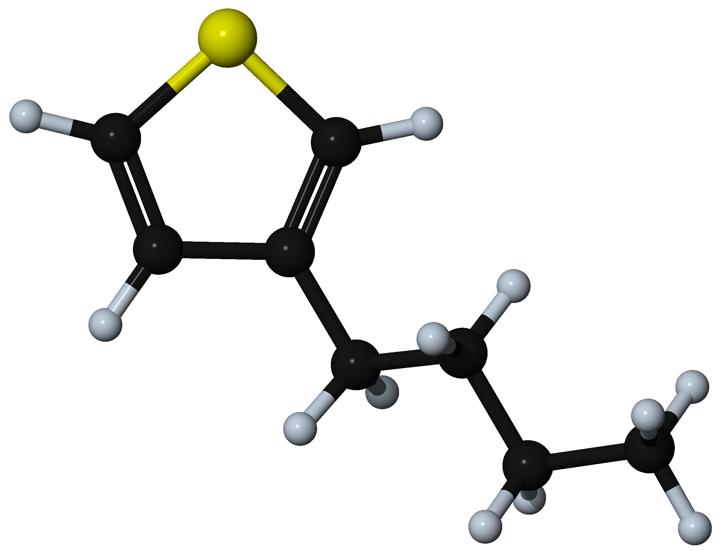
Then hydrogenate the model and add a suitable side chain to the thiophene ring, for example addition of a butyl substituent at the 3 position of the ring.
Now create the head and tail attachment points for the polymer chain. This is achieved by deleting hydrogen atoms at selected positions using the Atom >> Delete atom only command from the right-click context menu. This command retains the attachment point for fragment connection in the direction previously occupied by the hydrogen atom.
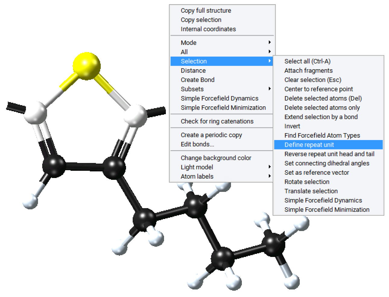
Once the attachment points have been created, select the atoms for these attachment points (and Selection >> Define repeat unit from the right-click context menu. One attachment point is then colored green, this is the head of the polymer backbone, and one atom is colored red, this is the tail of the polymer backbone. The Define repeat unit command determines the head and tail atom positions on the basis of atom ordering of the model. If you would like to reverse the head and tail positions, select the head and tail atoms, and use Reverse repeat unit head and tail command from the right-click context menu.
The newly defined repeat unit can now be employed in the Polymer Builder or exported to a user repeat unit library. To employ this repeat unit in the Polymer Builder, use the ‘get the repeat unit from a window in MedeA’ option to select the newly constructed fragment.
In the figure below, the resulting homopolymer is shown. Once constructed this polythiophene model can be employed in forcefield, semi-empirical, and first-principles calculations.
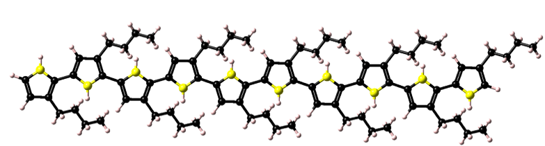
Structures with defined backbone flags can be saved for future use with the Polymer Builder by exporting MedeA.sci format files to your ~/MedeA/RepeatUnits folder. (Note, the name and location of this folder can be altered using the File >> Preferences… command). Hence any desired repeat unit can be constructed, saved, and employed in the MedeA Polymer Builder.
2.5.7. Random Substitutions

Use Random substitutions… to replace atoms and atomic masses in the current model, accounting for the current symmetry.
- generate a derived single structure (the default) or
- generate a set of derived structures (number of structures).
In framework structured materials, Lowensteins rule can be imposed and Al-O-Al linkages are forbidden. As a result, all aluminate tetrahedra must be linked to four silicate tetrahedral.
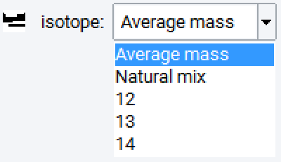
The substitutional rules employed are specified by applying the appropriate keywords in the set of rules shown on the dialog box. For example, by default the command exchanges all C atoms for Si atoms. This can be adjusted using the appropriate fields to so that either a percentage of C atoms are substituted, or a defined number of C atoms. You can also substitute atoms for vacancies and you can set the appropriate isotopic masses for any substitutions that you make.
Identical Random substitutions… dialogs are now employed in the MedeA interface and in the MedeA Flowchart interface. In the MedeA interface, the ‘Random substitutions…’ command is under Builders because the command generates new MedeA systems.
Note
with the MedeA HT-Launchpad license, this command can generate sets of derived structures as Structure Lists for use in high throughput calculations. Use Random Substitutions… from the Edit menu to replace atoms and atom masses in the current periodic model, respecting symmetry.
The isotope selector, shown here for Carbon, allows assigning known isotopes, average mass or the natural mix. This can be quite important to break the artificial periodicity for thermal conductivity computations; in this case perform substitutions for all atoms with the same element, but the natural mix for isotopes. Depending on the isotope distribution, the system size can be quite rather large to show some randomness in a given model.
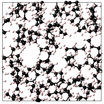
2.5.8. Amorphous Materials Builder
The MedeA Amorphous Materials Builder is designed for preparation of equilibrated models of disordered or partially ordered (oriented) organic or inorganic materials. Examples of typical systems are as follows:
- Molecular liquids and liquid mixtures
- Bulk rubbery or glassy polymers
- Polymer solutions and blends
- Lipid-like monolayers comprised of surfactants, counterions and solvent, etc.
- Slab-geometry film layers suitable for incorporation into interphase models
- Small molecule or polymeric systems with nematic liquid crystalline order
- Gas penetrant-organic or inorganic systems as encountered in membrane and coating applications
- Oxide and mixed-oxide inorganic glasses
Systems may contain an arbitrary number of components, each of which may consist of a system comprised of one or more atoms or ions, or a non-infinite bonded fragment or molecule obtained either from a standard MedeA .sci file, or from a model window in the current session. Individual components may be non-periodic systems, or periodic models with P1 symmetry. The overall molar composition is controlled by specifying the number of moles of each of the components, and options are provided to control whether molecules are treated as flexible, with rotatable backbone bonds, or as completely rigid units. Additionally, models may be prepared in the form of periodic infinite bulk cells, or with a confined layer geometry suitable for further manipulation to create monolayers or interfaces between dissimilar materials.
Main Dialog - Control Parameters
System geometry: permits specification of whether the builder will create a 3-D periodic ‘bulk cell’, or a periodic ‘layer’ system in which the Z-coordinates of atoms are biased to lie mostly within the current ‘c’ cell dimension. Note that in the latter case, since there is no absolute requirement that molecules reside entirely within the specified layer following the model building stage, a LAMMPS calculation beginning with a Compress Layer stage must be performed to complete the preparation and force all atoms to lie within the layer before using other building tools such as Stack layers… to create models of interfaces.
Specify cell…
Provides a variety of options for controlling the size of the amorphous models produced by the builder. Thus, for example, choosing Specify cell density will produce cubic cells in which the cell edges are determined based on the overall composition and density. Similarly, choosing Specify cell density,c will create tetragonal cells based on the density and specified c dimension, while choosing Specify cell a,b,c creates orthorhombic cells using the a, b and c lengths provided (in which case the density cannot be specified independently since it is fixed by the composition).
Control of cell dimensions can be useful when building a layer which will be used to create an interface with another layer whose cell edges are fixed (e.g. a crystal substrate). For convenience, the Cell details - density and edge lengths a, b, c - are displayed in a non-editable panel in the main dialog.
The full set of options for Specify cell … is as follows:
- density
- density,a
- density,b
- density,c
- density,a,b
- density,a,c
- density,b,c
- a,b,c
- Density
The desired density of the amorphous system in g/cm3. Required for all Specify cell … options except a,b,c.
Cell length (a OR b OR c): length of the given edge in Angstroms. Must be a positive real number.
Temperature: Temperature, in degrees Kelvin, for which the builder will attempt to create configurations which would be found with high probability in an equilibrium ensemble.
Coordinate bias: indicates that the positions of a pre-defined group of atoms, defined via an atom subset, will be biased to lie close to a specified set of grid points. Available options are as follows:
- none - disables the coordinate bias option
- 2D-grid - Randomly positions atoms from the specified subset on a two-dimensional grid displaced along the Z-axis of the cell by a user-specified distance. This feature can be used, for example, to locate surfactant head groups and/or associated counterions in an approximately planar arrangement (note that building such monolayers would usually also involve use of the layer System geometry control, together with the uniaxial Orientation bias option to preferentially align the tails of individual molecules).
- 3D-grid - Randomly positions atoms from the specified subset on a three-dimensional array of grid points, arranged symmetrically in the cell.
Usage of the coordinate bias option is subject to the following restrictions:
All components of the system must be of type ‘Rigid’ or ‘Pre-existing’ (see components panel parameter description below)
Individual molecules in the list of components should contain only one (or zero) atoms from the subset used to define the coordinate bias atoms
Grid dimensions: for 2-D grids, the grid contains nx*ny points, symmetrically arranged parallel to the XY plane of the cell, and displaced a distance z-offset along the Z-axis. 3-D grids contain nx ny nz points arranged symmetrically in the cell.
Coordinate bias subset: specifies the name of a subset identifying the atoms whose positions will be biased towards the positioning grid during model building. Note that the total number of subset atoms in all components included in the coordinate bias subset must not exceed the total number of available grid sites (nx*ny, or nx*ny*nz, as appropriate).
The subsequent equilibration of the partially-ordered models, using LAMMPS minimization and dynamics, will generally include an initial simulation stage in which the positions of the atoms in the coordinate bias subset are held fixed, to preserve the integrity of the ordered arrangement during the early stages of the equilibration.
The subset will normally have been defined within MedeA by selecting a single bias atom in each component to which coordinate bias will be applied (e.g. the sulfur of a sulfonate group), right-clicking to display the context menu, and selecting the Subsets >> Create subset from selection. Specification of a Subset name and clicking OK will then complete the definition of the subset for the given component. If molecules in other component windows contain atoms to be positioned using the same grid, the procedure is repeated, giving the same subset name.
Finally, if biasing using different grids is desired, the model building would be performed in two steps, with the first positioning one set of atoms, and the second incorporating the first model as a component of type Pre-existing, and applying the position bias to a second set of atoms using a different grid specification (to avoid later confusion, the second component’s bias subset would be given a different unique name). As an example, a monolayer model containing a surfactant and its counterions can be created by running the builder twice, such that the polyatomic anions are first incorporated by placing the head group atoms on a two-dimensional grid with z-offset value of, say, 6 angstroms (using the orientation option to align the tails), with a second invocation of the builder placing the appropriate cations on a grid with z-offset set to 2 angstroms, ensuring that the counterions are located in reasonably close proximity to the charged head group.
Orientation bias: applies an energy bias during system building to control the placement of specified groups of atoms. Available options are as follows:
- none - disables the orientation bias option
- uniaxial orientation - Biases the orientation of groups of atoms based on the specification of a pair of atoms that effectively define the orientation of the group as a whole (such as the first and last carbon atoms of each alkyl chain in the tails of rigidly-placed surfactant molecules, or atoms 4 and 4’ in the aromatic rings of the 1,1’-biphenyl group found in many liquid crystals).
- Direction
- When ‘uniaxial orientation’ bias is selected, specifies any vector along the preferred orientation direction. The vector does not necessarily need to be of unit length. Thus, for example, specifying values of 1.0, 1.0 and 0.0 for the ‘x’, ‘y’ and ‘z’ components will preferentially bias the orientation of parts of the molecules parallel to the XY face diagonal of the resulting periodic cell; similarly, specifying values of 0.0, 0.0, and 1.234 or 0.0, 0.0, and 1.0 will both bias the alignment along the Z direction.
Orientation bias pair subset: specifies the name of a set of atom pairs defining the intramolecular vectors desired to be preferentially aligned along the specified direction. Note that subsequent equilibration using LAMMPS must use this same subset in a protocol that preserves the original orientation to avoid the possibility of a loss of the orientation in some situations, such as equilibration at elevated temperatures or application of volume-changing methods such as NPT dynamics. Note that if the system contains more than one component, there is no requirement that the intramolecular vectors referenced by the given subset name should correspond to chemically identical units in the different components.
The pair subset will normally have been defined within MedeA by selecting a pair of atoms and accessing the context menu by right-clicking, followed by choosing Subsets >> Create to display the Create a subset dialog, within which a dynamic subset of length 2 (i.e. a pair subset) can be defined. See the documentation for a detailed explanation.
Number of configurations: is the number of statistically independent configurations of the amorphous system to create (each displayed in a separate window in MedeA). Generating a large number of configurations, whose properties can subsequently be averaged, may be essential when working with molecules whose conformations change infrequently during molecular dynamics simulation. This will generally be the case for high molecular weight polymers under ambient temperature conditions. Conversely, when simulating liquid and liquid mixture systems, generating a single configuration will be adequate, since molecular dynamics will usually explore a region of phase space sufficient to obtain meaningful average properties.
Main Dialog - Components Panel
The Components panel located at the top of the main Amorphous Builder dialog is used to specify a list of individual components which will be combined to create the amorphous model. Each component may be obtained from an already existing model displayed on the MedeA screen, or from a previously-created model stored in a structure file of type .sci. For each component, the following information must be provided:
Component: denotes the name of the component in the form of the name of a model contained in a MedeA window, or the name of a .sci file stored on the filesystem.
Type: components may each be one of four types:
- Rigid: During model building, all molecules of this type of component will be inserted as rigid units. If the Coordinate bias option is not used, the positions of molecule centers of mass will be chosen randomly. Otherwise the atoms contained in the Coordinate bias subset are placed according to the selected grid. Similarly, if Orientation bias is not used, molecule orientations are chosen randomly, as opposed to being subjected to the specified orientation bias. In all cases of rigid placement, internal bond conformational angles remain exactly as in the original component.
- Flexible: In the case of flexible molecules with many internal torsional degrees of freedom, it is generally desirable to sample all energetically reasonable dihedral angles within a component molecule. Unless the component is found to contain zero rotatable bonds, this option will force sampling of all internal dihedrals formed by all sequences of non-hydrogen atoms within the component.
- Auto: Specification of this component type indicates that the builder should decide automatically whether intramolecular dihedral angles will be sampled during model building.
- Pre-existing: This option is used whenever the new system is to be created by adding more material to an already existing model - e.g. adding small penetrant molecules to an amorphous model for diffusion studies, or solvating a system with a much larger quantity of solvent to create a dilute solution or interfacial model. Note that inclusion of a pre-existing model in the list of components will automatically select the ‘a,b,c’ Specify cell mode, and set the number of copies of the component, Nmols, to 1. The a,b,c parameters of the pre-existing model then define the cell parameters of the new model. Finally, note that in contrast to the restrictions applicable to components of type rigid, flexible and auto, a pre-existing component type may include infinite covalent networks such as those created using the MedeA Thermoset Builder.
Nmols: specifies the number of moles of the component in the final amorphous model (i.e. per mole of cells). Note that if the component is of type Pre-existing, the number of moles of this component will be set automatically to 1, since multiple spatially identical copies of a component is not permitted.
Relax: following the initial building, the amorphous model will normally be subjected to pre-equilibration to prepare for subsequent simulation (e.g. using MedeA LAMMPS). Unchecking the Relax toggle can be used to disable this relaxation during pre-equilibration, which will prevent changes in coordinates of atoms whose original positions should be preserved. Examples include the building of solvated systems in which the solvated molecule must be left in its original conformation or, analogously, hybrid systems consisting of an immovable crystalline component interfaced to a mobile phase.
Hint
If this fixing of atoms is to be continued into subsequent simulations, it may be helpful to define the fixed portions of the system as one or more subsets prior to amorphous model building.
2.5.9. Thermoset Builder
The models created by the amorphous builder are the starting point for creating thermosets. There is no interactive way to deal with these larger models, which are handled through flowcharts and described in detail in II.F. 5. 5. Thermoset Builder.
2.5.10. Stack Layers Builder
The MedeA Stack Layers Builder is designed for preparation of interfacial systems comprising two or more layers of materials. Individual layers may be amorphous or crystalline solids, liquids, partially-ordered liquid crystal systems, and vacuum regions (empty cells) if so desired. The layer builder itself can process any type of material - organic, inorganic or metallic, though the feasibility of subsequent simulations will require that the chosen simulation tool supports all components of the combined system (e.g. for classical simulations, the forcefield used must include coverage for all atoms and interactions within the model).
In order to use the stack layers builder, it is a requirement that none of the component layer systems contain bonds that cross the top/bottom faces of the cell. Suitable models can be prepared by combining the System geometry: layer option of the Amorphous Materials Builder with a Compress Layer LAMMPS equilibration flowchart stage (note that the Amorphous Materials Builder layer option itself is not intended to create models completely free of bonds crossing the cell ab faces, rather it only applies a bias to confine material mostly within the layer). Alternatively, layer systems used as input to the stack layers builder can be created manually or using other MedeA tools such as Interfaces.
Regardless of the method used to create the component layer, it will usually be advantageous to ensure that all layers have been pre-equilibrated, since this will minimize the risk of disruption of the newly-created interface(s) during subsequent simulations owing to the presence of unduly large forces on atoms in the interfacial region(s).
When the Stack Layers Builder is first invoked for a periodic system from Builders >> Stack layers…, the dialog panel shows entries for two component layers. By default, the currently-active MedeA model system is pre-selected as the first (‘topmost’) layer of the new system, though this can be changed if desired simply by clicking on the name and choosing a different system from the list provided. The second layer of the new system is then specified by clicking on ‘Select System’ and choosing from the list provided. Any number of additional layers may be added by clicking the Add Layer… button and repeating the selection steps. Finally, when the OK button is pressed the new layered system is created with layers in the order specified in the dialog and displayed on the screen with the Z-axis oriented vertically.
Main Dialog Parameters
The Layer System: specifies the system to be used to create individual layers. Clicking on this entry displays a list of eligible P1 models.
The Subset parameter specifies the name of a subset containing atoms from the layer that will be made part of the created layer model. If subsets are not required, this entry may be cleared and left blank.
Adjust offers precise control over the distance between the top most atom in a layer and the lowest atom in the layer immediately above. Clicking on … will open the Layer Data dialog, which provides for adjustment of the layer prior to building the final multilayer system. Details of available adjustment options are given in the adjust parameters section below.
The Add Layer… adds a new row to the Layers panel. Parameters for each additional layer are then specified in the same manner as already performed for the layers higher in the stack. Layers beyond the second in the multilayer system include a Delete button for removal of the layer if necessary.
Layer Data Adjust Dialog Parameters
The Preadjust layer: allows input of additional data to control the thickness of the layer when the multilayer system is finally assembled.
The Preadjust layer to atoms +: specifies a distance in Angstroms which will be added to the thickness of the layer after first setting the thickness of the layer cell to the value defined by the difference between the highest and lowest Z-coordinates of atoms in the component layer. This can be useful to exert precise control over the minimum separation between atoms in two adjacent layers.
For example, specifying preadjustment distances of say 4 Angstroms in each of two adjacent layers will guarantee that in the resulting multilayer system, no atoms approach closer than this distance. Note that the preadjustment space is apportioned equally at the top and bottom of the cell (i.e. the Z coordinates of the component layer atoms are effectively first centered in the cell, and then shifted upwards by one half of the distance specified).
Finally, note that if the pre-adjust option is used with an empty cell to insert a vacuum layer, since there are no atoms present, the thickness of the inserted layer will become that of the Preadjust layer to atoms + parameter itself.
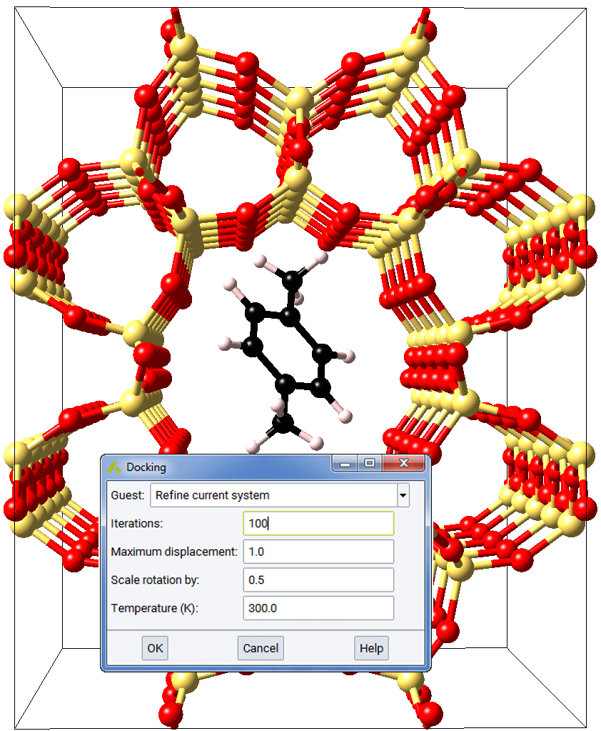
2.5.11. MedeA Docking
The computational analysis of the preferred orientation of one molecule in the environment of a second structure, which may be a surface or a microporous material is generally termed ‘docking’ [1].
The MedeA Docking command, invoked from Builders >> Docking… for a periodic system, facilitates the creation of composite models. The command takes an existing bulk system and merges into this system a specified second structure. If the current system already contains a host-guest complex, this combined system may be optionally refined using the Docking command.
The docking algorithm employs the Metropolis Monte Carlo algorithm [2] to sample possible configurations for the second system relative to the specified host system. For each trial configuration the energy change required to create this configuration is used to compute a Boltzmann probability and this is compared with a random number between 0 and 1 to either accept or reject the changed configuration. Reducing the simulation temperature allows the docking process to reject energy increasing moves and increasing the temperature causes energy increasing moves to be accepted.
The energy of trial configurations is evaluated through the use of a simple 12-6 Lennard-Jones potential. This simple description allows the command to provide sterically plausible structures. The relative energy of possible configurations is only a first approximation and more elaborate forcefields or quantum mechanical methods should be employed in evaluating the energetic properties of composite systems.
2.5.11.1. Docking Dialog Input - Required Parameters
Guest: The guest system to be introduced to the current system by the docking process. The docking procedure creates a new system, with Host and Guest subsets. Note that if the current system already possesses Host and Guest subsets, the current Host-Guest complex may optionally be refined.
Iterations: The maximum iterations to be employed in the Monte Carlo docking process.
Maximum displacement: The maximum displacement to be applied to the guest system in Angstroms.
Scale rotations by: A scale factor applied to Euler angles of rotation
applied to the guest system at each iteration. Random Euler angles are
chosen in the ranges  ,
,  , and
, and  . The scale
factor is applied to each rotation to limit angular sampling.
. The scale
factor is applied to each rotation to limit angular sampling.
Temperature (K): The temperature in degrees C employed in the Metropolis Monte Carlo procedure. Selecting a high temperature will cause high energy structures to be accepted in the Monte Carlo search process, and a low temperature will favor energy reducing configurations.
2.5.11.2. Docking - Notes
The initial configuration employed in Docking locates the guest molecule at the center of the Host system. This configuration may be of high energy and several iterations may be required to find more reasonable steric configurations.
Hint
Docking may be interrupted with the Escape (Esc) key. The final configuration is always that of the lowest energy configuration sampled during the current docking process.
The MedeA docking functionality can be employed in interactive building as described above. In addition, docking is implemented as a flowchart stage, which permits the combination of host structures with guest configurations obtained from molecular dynamics trajectories as a part of computational workflows employing flowcharts.
2.5.12. Special Quasirandom Structures
Special Quasirandom Structures SQS are good models for disordered alloys, as the coordination number in the different coordination shells are identical to or close to those of a random, disordered alloy with a given stoichiometry. MedeA allows building such structures from the Special Quasirandom Structures (SQS)… entry of the Builders menu.
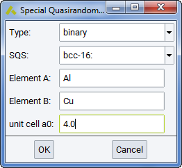
The first selection is the Type of binary, ternary or pseudoternary alloy.
Then you select as SQS one individual structure (like the A3B) or an entire set for a given lattice type and size (the bcc-16 series of bcc structures with 16 atoms).
The required inputs are elements A, B, and C (only for ternaries) and the lattice constant a 0.
Binary alloys: bcc, fcc, hcp
MedeA offers 8-atom models for bcc and hcp structures, 16-atom models for bcc, fcc, and hcp; 32-atom models for fcc. This means you create the A3B, AB, and AB3 for a given lattice constant at once. That’s even more impressing and timesaving with getting all 15 fcc models with 32 atoms each.
More details on these quasirandom structures in general and the binary structures are for example from Wolverton & Ozolins [4] and Zunger, Wei, Ferreira & Bernard [5].
Ternary alloys: fcc, bcc, B1
fcc: ABC (24 atoms) and A 2BC (24 atoms): Shin, van de Walle, Wang & Liu [6]
B2: A 2BC (8 atoms), and A 4B 3C (16 atoms): Jiang, Chen & Li [7]
bcc: ABC (36 atoms), A 2BC (32 atoms), A 2B 3C 3(64 atoms) and A6BC (64 atoms): Jiang [8]
Pseudoternary alloys: Zincblende-64
A variety of different stoichiometries realized by structures with 64 atoms
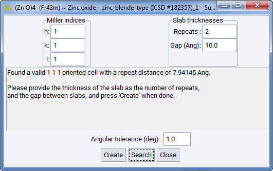
2.5.13. Build Surfaces
The MedeA Surface Builder lets you build surfaces from bulk structures by defining a set of Miller indices.
- Start from a periodic bulk structure
- Invoke surface builder through the MedeA menu entry: Builders >> Build Surfaces…
- Select Miller indices (e.g. 111) and press Search
- Follow the instructions printed by the surface builder to build your surface model
The following options and parameters are available:
2.5.13.1. Orientation and Thickness
- The Repeats: setting varies the material thickness by changing the number of cells to stack in the direction of the surface plane
- The Gap: setting sets the thickness of the vacuum layer. The default of 10 \({\mathring{\mathrm{A}}}\) is a good value making sure that there’s no interaction between surface layers within the periodic boundary model used e.g. by VASP
- The Angular tolerance: setting sets the allowed devation of the surface normal from the desired direction. This is needed for some bulk structures and surface as it is not possible to build a coherent cell accommodating the structure with correct stoichiometry.
- The Create: button builds and displays a preview of the surface model
MedeA now displays a preview window allowing you to set further parameters and to check the symmetry of the resulting system before building the final structure.
2.5.13.2. Surface Builder Preview Window
Here, you can verify the model, check its symmetry and possibly move the surface plane to cut parts of the structure away and modify terminations.
- Use the sliders Plane 0 and Plane 1 to remove surface layers. For example, in hexagonal ZnO above, you may decide to terminate both surfaces by just zinc atoms or by just oxygen
- Click Update to display the current symmetry
- Click Reset to return to the previous builder screen
- Click P1, Symmetric or Centered P1 to choose in which symmetry to display the final system
- Click Apply to create the final surface structure but keep the Preview window open
- Click OK to create the final structure and close the Preview window
- Click Cancel to abandon the whole operation
Note
Changing the termination of the slab model may change the stoichiometry and symmetry of the system. If your goal is to calculate the surface energy you should make sure that both surfaces present in the slab model are identical. Also, in polar systems, you may want to avoid creating a dipole by working with systems that have inversion symmetry.
What symmetry you choose for the final surface depends on your goals: For example, to calculate the surface energy of the above system you would like to use the full symmetry of the system. To add a molecule to the surface, you most likely would use P1, as you are going to further modify the structure.
- Create as P1 creates a slab model exactly the way you see it on the screen
- Create as Symmetric uses the new symmetry to set up the slab model, might change the cell shape
- Create as Centered P1 creates a slab model as you see it on the screen, but re-centered
2.5.14. Build Supercells
The Supercell Builder lets you create a large cell starting from your initial periodic structure.
- Invoke the supercell builder from the MedeA Builders menu item Build Supercells….
The following settings are available:
| Mode | Description | |
| Simple | Increases lattice parameters in a, b, and c direction Also available as a flowchart stage |
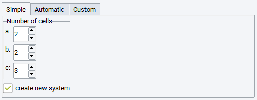 |
| Automatic | Uses range parameter to build a supercell: i. Extension equally in all directions ii. Extension in one direction |
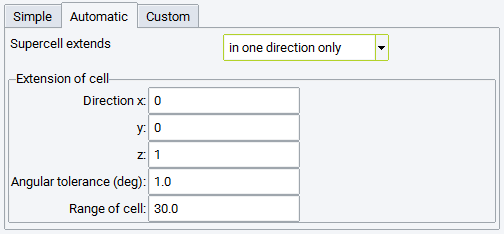 |
| Custom | Defines a new set of lattice parameters for supercell | 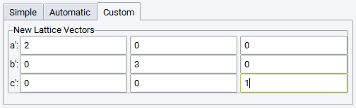 |
2.5.15. Context Sensitive Menu for Molecular Structures
Right-clicking into the drawing area of the Molecular Builder interface brings up a context sensitive menu. The following list describes the available options:
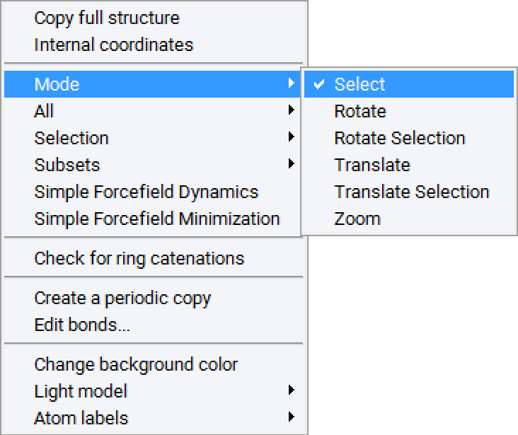
The Mode menu
The mode menu lets you select an action mode. Current modes are Select, Rotate, Rotate Selection, Translate, Translate Selection and Zoom. Alternatively, the Insert mode is invoked by selecting an element from the insert panel or by clicking the Insert icon in the MedeA menu bar.
Right-click to use context sensitive menus
All other modes are selected through the context sensitive menu or through menu buttons in the Molecular Builder menu bar. The cursor shape indicates the current viewing mode:
 for Insert
 for Select
 for Rotate and
  for Rotate Selection
 for Translate and
  for Translate Selection
 for Zoom
In addition, the MedeA menu bar displays buttons for selecting modes when a molecular builder window is active:

Move your mouse cursor over these buttons to display a brief description of each mode.
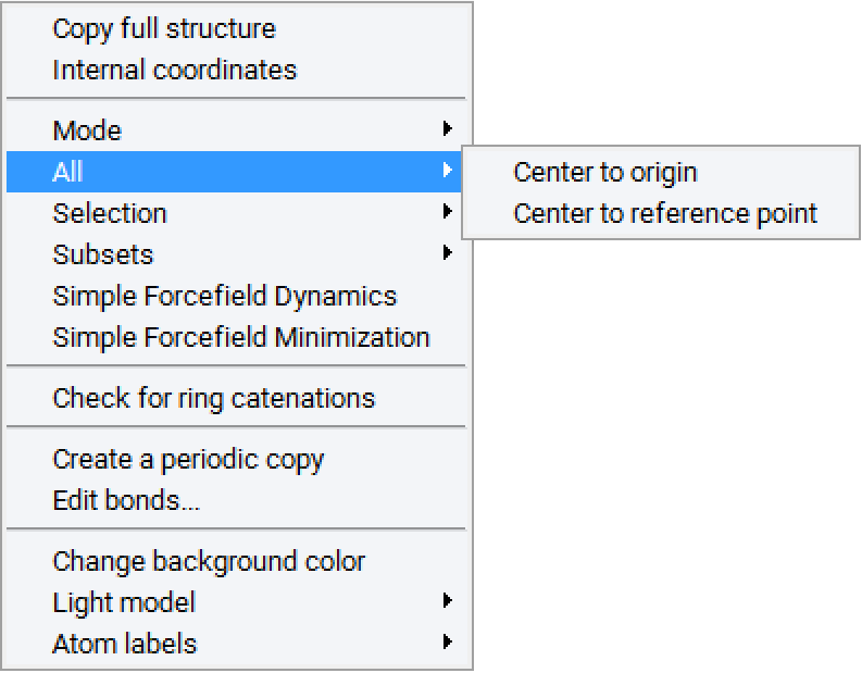
The All menu
The All menu lets you center all atoms in the drawing area to either the origin or to the origin or a reference point of your choice. Centering means moving the center of the smallest box which envelopes all atoms (bounding box) to the reference point/origin.
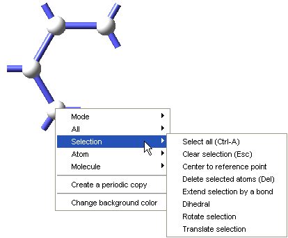
The selection menu
The selection menu lets you perform a certain operation on a selection of atoms. Available operations depend on the number of selected atoms:
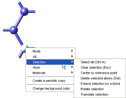
When one atom is selected
- Select all - Selects all atoms in the drawing area (shortcut Ctrl-Alt)
- Clear selection - Unselects all selected atoms (shortcut Esc)
- Center to reference point - Moves all atoms present in the drawing area such that their geometric center comes to lie at the reference point. Defining a reference point.
- Delete selected atoms - deletes all selected atoms (shortcut Del)
- Extend selection by a bond - Adds all atoms connected to the selected ones
- Rotate selection - Rotates the selected atom around the reference axis. A dialog will ask for the rotation angle
- Translate selection - Translates the selected atom by norm (reference vector) along the reference vector
When Two Atoms are Selected (Only Options not Mentioned Earlier are Listed)
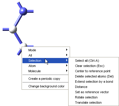
- Distance modifies the distance between two atoms, choose which to move
- Set as a reference vector - Sets the bond connecting the two selected atoms as a reference vector
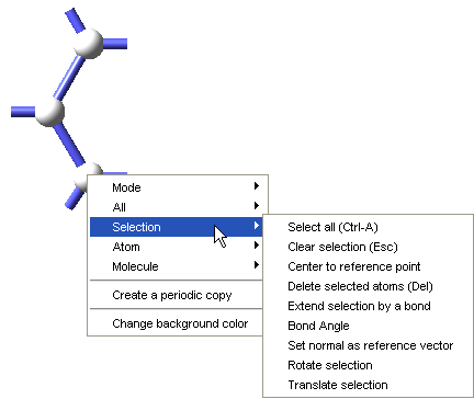
When three atoms are selected (only options not mentioned earlier are listed)
- Bond angle - Displays dialog to view and edit the bond angle including the option change which atom to displace when changing the angle
- Set normal as reference vector selects reference vector normal to plane spanned by three atoms
When Four Atoms are Selected
- Dihedral - Displays dialog to view and edit the dihedral angle including the choice which of the two atoms at the end of the chain to displace when changing the angle. This option requires 4 linearly bonded atoms
Right-Click When Cursor over a Bond Dividing the Molecule
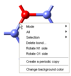
- Delete bond… - deletes the bond
- Rotate <atom_number>side - rotates the part of the molecule connected to <atom_number> around the bond (when atoms are selected)
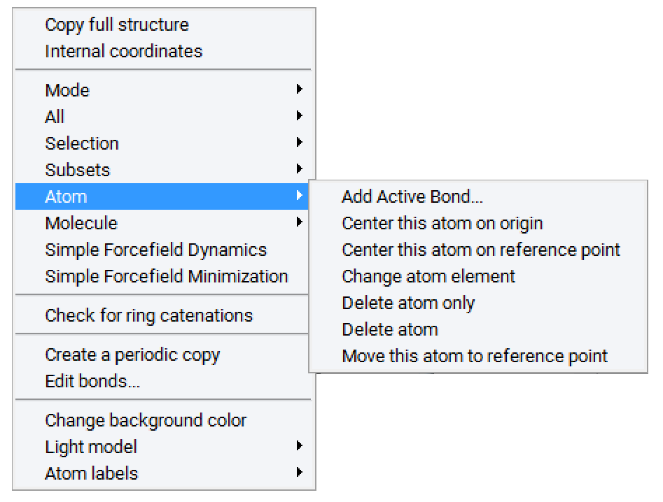
When Right-Clicking on an Atom (Only Options Not Described Earlier are Listed)
- Add active bond - Creates an active bond perpendicular to the current viewing plane
- Center this atom on origin - Moves all atoms such that the atom under the cursor comes to lie at the origin (0,0,0)
- Center this atom to reference point - Moves all atoms such that the atom under the cursor comes to lie at the reference point
- Change atom element - replace the element under the cursor by the element currently loaded into the cursor
- Delete atom only - Deletes the atom leaving the active bonds of the atom(s) bonded to this atom
- Delete atom - Deletes the atom and all bonds connecting to this atom
- Move this atom to reference point - Moves only the atom under the cursor to the reference point
When right-clicking on an atom - Molecule
In the following, “Molecule” refers to all atoms connected to the one under the cursor.
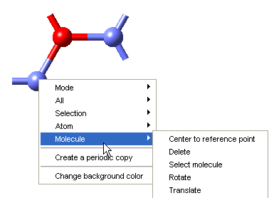
- Center to reference point - Centers the molecule to the reference point
- Delete - Deletes the molecule
- Select molecule - Selects the molecule
- Rotate - Rotates the molecule around the axis defined by Point and Vector
- Translate - Translates the molecule by the vector defined by Vector
Right-Click Anywhere in the Drawing Area - Create a Periodic Copy
- Create a periodic copy of the molecular system, which can be used as input for e.g. VASP
Save as a Fragment
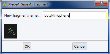
Save as a fragment - Molecules that have exactly one active bond can be saved as fragments for later use as a building block for more complex structures. When saving a fragment make sure to choose a comprehensive name and in the graphics panel zoom in on the fragment beforehand. MedeA will save a snapshot of the structure along with its name
Tip
This option is shown only when the structure has exactly one active bond!!
Shortcuts
A number of shortcuts are available to simplify operations:
- Ctrl-M - invokes the Molecular Builder interface for a new system
- Ctrl-A - Selects all atoms in the drawing area
- Ctrl-Z - undoes the last action
- Esc - Clears the atom selection
- Del - deletes all selected atoms
- R/T/S/Z - press and hold down one of these keys to temporarily swap between the current mode and Rotate/Translate/Select/Zoom
- R/T/S/Z + \(\leftarrow\)\(\rightarrow\)- Rotation of 1 0/Translation of 0.1 \({\mathring{\mathrm{A}}}\) Zoom
- R/T/S/Z + Shift + \(\leftarrow\)\(\rightarrow\)- Rotation of 10 0/ Translation or 1 \({\mathring{\mathrm{A}}}\) Zoom using larger steps
- S+/R/T + \(\leftarrow\)\(\rightarrow\)or left-mouse-click - Rotates/Translates selected atoms; Rotation around current vertical axis
- S+/R/T + \(\uparrow\)\(\downarrow\)or left-mouse-click - Rotates/Translates selected atoms; Rotation around current horizontal axis
Adding ALT to the above commands translates or rotates along the axis perpendicular to the view plane
2.5.16. Substitutional Search
2.5.16.1. Features and Algorithm
MedeA’s Substitutional Search takes the active structure window as an input and searches all symmetrically different systems obtainable by substituting an element in the system by an other element at the same site. A vacancy can be chosen as the type. The maximum number of allowed substitutions is half the number of atoms of the type already present in the system.
The search algorithm proceeds as follows: First, a single substitution is made for each symmetrically independent site A, hereby generating a set of new structures. The structures resulting from this operation are grouped by their new symmetries. Next, for each element of the new set of structures, a second substitution is performed on each symmetrically independent site; again the resulting structures are regrouped according to symmetry, and the process is repeated up to the desired number of substitutions.
2.5.16.2. Usage
To bring up the Substitutional Search interface, select the periodic structure window you would like to perform the search in and select Substitutional Search from the Builders menu:
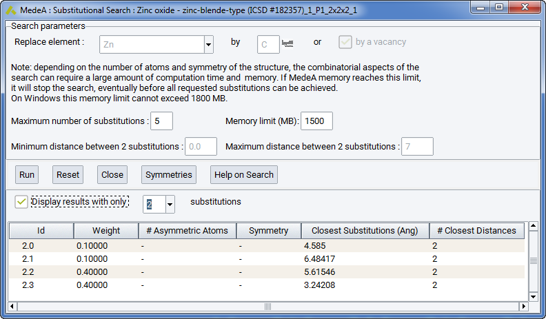
To start with, select which element to replace (here: Zn) and select an element to replace by (here: vacancy). You can use additional parameters to limit the search, e.g. by defining a minimal or maximal distance between two substitutions.
- Run: Starts the Search
- Reset: Resets the search without changing the parameter settings
- Symmetries: Calculates the symmetries for all structures displayed in the results table
- Help on Search: Brings up help text on Substitutional Search
In the previous example of up to two vacancies in ZnO having a maximum distance between two substitutions of 7 \({\mathring{\mathrm{A}}}\) clicking Symmetries creates information on the number of asymmetric atoms per cell and the cell symmetry:
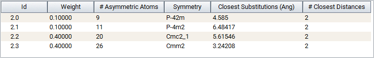
Search results are listed in the results table and classified by an Id number giving the number of substitution in the system followed by an index. For example, Id = 2.1, 2.2, 2.3, 2.4 means that 4 symmetrically different systems with two atoms replaced by atoms have been found.
The displayed results can be filtered by the number of substitutions per system, check Display results with only [n] substitutions and select a number for substitutions
The table can be sorted by right-clicking on a column header and selecting a sorting criterion.
Right-click on a structure entry to view a structure, compute its symmetry or copy the system to an internal buffer for later pasting to a Combi Spreadsheet.
Other Search options are:
Replace element [ ] by [ ]: Element to be replaced () and element to substitute with ()
Maximum number of substitutions:to be performed (default=5)
Memory limit (MB): The memory limit in MB to be imposed for the search (see explanation in the panel text).
Minimum distance between 2 substitutions: Only systems having a distance between substitutions larger than this parameter are considered (default=0)
Maximum distance between 2 substitutions: Only systems having a distance between substitutions smaller than this parameter are considered (default= not set)
2.5.17. Merge
Merge combines the contents of two periodic structures, and is invoked from Builders >> Merge… for the larger model. The second model is translated by x, y, and z (units in Angstrom).
If the two models don’t share the same lattice vectors, you can shift the second system in the bigger first system, as defined by a translation vector. Please take care that the second system has smaller or equal dimensions than the first model.
2.5.18. Building Interfaces
2.5.18.1. Features and Algorithm
The MedeA Interface Builder takes one or two surfaces slab structures as an input. It then searches for a relative orientation of these two surfaces such that the lattice mismatch in the resulting system is minimized.
- For each of the surfaces, loop over the allowed range of cells, creating new cells that are multiples of the original cell: a’ = ma + nb, b’=oa + pb where a and b are the original in-plane lattice vectors and m, n, o and p are integers from -max to +max
- For each cell find the reduced cell, which gives a standardized list of possible cells
- Find the matches between the two lists of reduced cells that meet the requested tolerances for the mismatch of the area, lattice parameters and angle
- Build the surface structures for the reduced cells that match, testing for and removing duplicates. These are saved in the subdirectory surfaces
- Build the trial interfaces from the surface structures
- Find the reduced cells for the interfaces, looking for translational symmetry
- Compare the reduced interface with previous ones and remove duplicates
As a result Interface Search produces:
- A spreadsheet of interface structures with geometrical parameters that can be used for visualization, further geometry and symmetry analysis and as an input for computations
- A subdirectory ./interfaces (in the job directory, accessible through Job Control) containing all interfaces using default parameters for gap sizes and \({\gamma}\)-surface shifts
- A subdirectory ./surfaces containing all surface structures built from the reduced cells that matched the tolerance criteria
2.5.18.2. Usage
Here are the steps required to create a set of interfaces:
- Prepare two surface models using the surface builder. You can also use a single surface model to make a grain boundary
- Select Interfaces from the MedeA Tools menu. A new entry Interfaces will appear in the MedeA main menu:
- Make one of the surfaces the active system in MedeA
- Select Define and Run from the Interfaces menu. The interface search dialog is displayed:
2.5.18.3. Default search parameters
By default, the algorithm looks for interfaces between the active, selected surface and itself (shown as the default setting for Second System). A tolerance of 5% will be allowed for the misfit of the area, length and angle of the two new subsystems respectively.
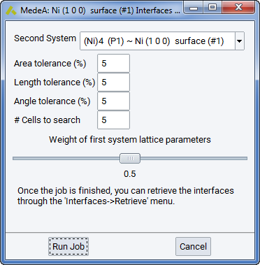
A plane which is in-plane with the selected surfaces area(s) and has the size of 5x5 the original surface cell(s) will be searched for Bravais-type lattice vectors making up the new cell and complying with the mismatch tolerances.
In order to make a coherent cell, the in-plane lattice parameters of the two cells need to be adjusted. By default the interface builder weighs the lattice parameters of each system with a factor 0.5, meaning both systems will be dilated/constrained by the same amount. In general you may choose a weighting factor depending on your knowledge about the elastic properties of the two materials involved.
2.5.18.4. Description of Search parameters
Second system: Opens a dialog to select the second system from the list of structures currently open in MedeA. The second system can be identical to the first one, for example when searching for grain boundaries.
Area tolerance (%): The tolerance for the deviation between the two native surface areas making up the interface. Here, “native” means “by construction”, that is before applying any strain to fit the two surfaces together.
Length tolerance (%): Tolerance for mismatch of the natural in-plane lattice parameters of the two surface cells.
Angle tolerance: Tolerance for the mismatch of the natural in-plane angles of the two surface cells.
#cells to search: How many multiples of the original cell to use for constructing new surfaces during step 1 of the search procedure (see algorithm above)..
Weight of first system: Determines how much strain (between 0 and 1) is applied to the first system, when fitting the two surfaces together to form an interface. The remaining weight will be applied to the second system.
Click Run to submit the interface search job.
Building the new surface structures, finding the reduced cells and symmetries and constructing and comparing the interfaces may take a considerable amount of CPU time. Depending on input symmetry, search space and system size, time to completion can vary between minutes and hours.
2.5.18.5. Display of results
In order to show the results of a completed interface job, invoke Retrieve from the Interfaces menu entry.
Select the interface job in question from the file selection dialog and click Insert and then OK. You will get a spreadsheet-like window showing the data of those systems that fulfill your tolerance criteria. The screenshot below shows an example of Interfaces default output for (100) Ni twist grain boundaries. The following table summarizes the parameters given in the output:
Identical Interfaces: (Yes/No) indicates if the two interfaces present in the cell are identical. Using a structure model having identical interfaces allows for direct calculation of e.g. the interface energy. Given that the Interface Search works with 3D period or crystalline structures, a slab model of an interface has to have two actual interfaces in a unit cell.
ID: Counts the class of the interface, followed by another index, if there are different interfaces in this class. In the example below, the class 1 has two interfaces with different symmetry.
nAtoms: The number of atoms in the interface unit cell.
Space group: Symmetry of the resulting interface unit cell.
Area (AA): Area of the interface in AA2
dA: Area mismatch of the two natural surfaces making up the interface.
A, B, dA, dB: A and B lattice parameter of the interface, the mismatch of the original (natural) lattice parameters A and B in %.
Theta, dTheta: The angle of the 2-D cell (in-plane angle), the mismatch of the original (natural) in-plane angles
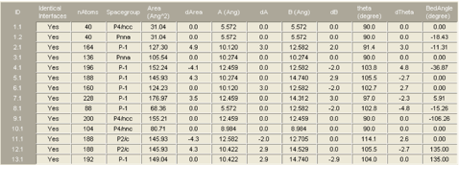
Bed angle: The twist angle between the two surface layers making up the interface
To create an interface for one of the listed structure parameters, select a row in the spreadsheet, right-click and select Create interface to bring up a preview window with a number of additional options for the construction of the final interface structure.
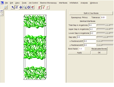
The above preview window provides a number of additional options for building the final interface structure:
Split in two surfaces - Lets you split the interface into the two corresponding subsystems (surfaces). Use this option when calculating e.g. the work of separation for an interface
Spacegroup/Tolerance - Shows the current symmetry and lets you modify the tolerance used to calculate symmetry. Click Apply to recalculate symmetry.
Identical interfaces - Indicates if the two interfaces present in the cell are identical.
Total/upper/lower gap/Gap ratio - allows you to define two independent gaps for the upper/lower interface.
x,y fractional shifts - Lets you move the two substructures making up the interface in a plane parallel to the interface. Use this option to create additional points on the so-called \({\gamma}\) -surface.
Bond factor / Recalculate bonds - Lets you apply a bond factor and recalculate bonds for the interface.
Apply - Applies changes to the interface structure.
2.5.19. Conformers Search
Computing some properties may require considering all molecule conformers or at least a set of most representative conformers when they are too numerous. Identifying the interesting conformers of a molecule or set of molecules requires specific search and minimization routines. This tool is invoked from Builders >> Conformers search… and allows you to search molecule conformers, that can be chosen from MedeA windows or a file, containing a single molecule.
As an alternative, a SMILES string, that is quite commonly used and a convenient way to describe a molecule. SMILES stands for Simplified Molecular Input Line Entry Specification: specification in the form of a line notation for describing the structure of chemical molecules using short ASCII strings. The dialog allows you to type in or copy a SMILES string.
Once the molecule of interest is provided, the number of possible conformers is indicated (if this number is higher than 100,000,000 it will be simply mentioned so). According to this number a search strategy is automatically set and one just needs to press “Find Conformer”. The search time depends on the complexity of the molecule, depending on the number of rotatable bonds and their number of local energy minima they have. When completed the resulting list of conformers is displayed in a table in the Results tab. The first of the list is the most stable conformer found.
The SMILES conversion and conformer search is performed by a separate program called automatically by MedeA. This program is built with the OpenBabel library (see http://openbabel.org) and is licensed under the GPL conditions. This program follows the conditions of this license. The forcefield used for the search is the UFF94 that is applicable to a wide variety of molecules, so the conformers energies have to be understood relatively to this forcefield.
The available conformer search strategies are the following:
- Systematic: search all possible conformers, rotating torsions step by step. This is suited for a small number of conformers.
- Weighted: randomly rotates around the rotatable bonds in a molecule, the random choice of torsions is reweighted based on the energy of the generated conformer.
- Genetic Algorithm (GA): optimize the conformer energy using the UFF94 forcefield and preserve diversity in terms of different torsions values on rotatable bonds.
When the number of possible conformer is small, MedeA will selects automatically the systematic search, if not the GA will be selected. But one can freely select the parameters through the advanced options.
For systematic or weighted search, the conformers in the list are sorted as a function of their conformer energy (UFF94). For the GA search, the following conformers are added according to their similarity with the previous conformers in the list. The similarity is a distance, which is defined by the number of different torsion values with respect to previous conformers. Similarity of 0 means identitical.
Additional column provides:
- Similarity to first: similarity to the most stable conformer
- Average similarity: average similarity to all other conformers in the list
- Minimum similarity: minimum similarity to all other conformers in the list
2.5.20. Structure List Editor
Define a list of structures, with arbitrary configurations and compositions. Structures can be simple molecules, molecular fluid or solids. These lists are stored in a single file and allow to leverage the power of flowcharts to handle automatically a large number of molecules.
This dialog is invoked from File >> Structure List file… and allows you to create new lists and browse and edit the existing ones. You can then add a selection of structure from MedeA, from files or appending another list. Alternatively, you can use a list of SMILES strings (see Conformer Search for a description) from a file containing one such string per line eventually preceded by its name, e.g.:
Alanine CC(N)C(=O)O Caffeine O=C1C2=C(N=CN2C)N(C(=O)N1C)C Valine CC(C)C(N)C(=O)O Leucine CC(C)CC(N)C(=O)O Tyrosine NC(Cc1ccc(O)cc1)C(=O)O
You can later rename and delete structures from the list and also export all or a selection to individual files (1 per structure) using a common file name prefix.
Then the purpose of such lists is to be used in Job Flowchart where they can be selected in a “Structure List Loop” stage, that will apply the same sub flowchart to all or selected structures from the list. A more detailed description of structure lists is given in the Medea| HT section.
2.5.21. Generic simple Forcefield (Minimization and Dynamics)
A generic simple forcefield is defined in MedeA to add the ability to clean (remove local stresses caused during building or construction) the active system. It is of a very generic form, covers all elements, and works with any system in MedeA.
It is defined with the following components:
- bonding potential: when 2 atoms are bonded, a reference bond length is defined as the sum of the valence radii, and the potential is proportional to the square deviation. If the bond order is aromatic, double or triple a reducing factor is applied to the reference length.
- bond angles potential: the potential is proportional to the square deviation from a target angle. The target bond angle is determined in a generic way according to the number of bonds and order, e.g. 120 degrees for 3 single bonds.
- improper torsion: only defined for atoms having 3 bonds, will be minimal when the atom is in the same plane as its 3 connected atoms.
- non bonds interaction: following a Lennard-Jones 6-12 form. Parameters are adjusted to fit the sum of Van der Walls radii
- electrostatic charge: a small positive charge is added creating an additional repulsive potential.
Because of their simplicity these potentials cannot be effectively fitted (individually or as a whole) to reflect actual energy values. The default constants are determined empirically to maintain a good overall balance.
The generic simple forcefield is used for structure clean-up and optimization in two different manners, both available from the right-click context menu of a molecular or periodic P1 structure, and as a flowchart stage:
Simple Forcefield Minimization: perform a fast and interactive geometric optimization to avoid close distances or long bonds. This will not necessarily provide highly accurate geometries, but in most cases it will provide a good starting point to search for it.
Simple Forcefield Dynamics: start with a pseudo molecular dynamics (not strictly defined temperature since the forcefield uses a crude energetic presentation only) for a limited number of steps followed by a geometric optimization. It can be applied repeatedly and displays intermediate conformations to illustrate the current geometry of the system. This option can be useful to relax a set of molecules or a single large molecule.
Note
If the result of Simple Forcefield Minimization or Simple Forcefield Dynamics does not match expectations, you can simply undo (ctrl-Z) any structural changes.
| [1] | Thomas Lengauer and Matthias Rarey, “Computational Methods for Biomolecular Docking,” Current Opinion in Structural Biology 6, no. 3 (June 1996): 402-406; D W Lewis, Clive M Freeman, and C Richard A Catlow, “Predicting the Templating Ability of Organic Additives for the Synthesis of Microporous Materials,” Journal of Physical Chemistry 99, no. 28 (July 1995): 11194-11202; Dewi W Lewis, David J Willock, C Richard A Catlow, John Meurig Thomas, and Graham J Hutchings, “De Novo Design of Structure-Directing Agents for the Synthesis of Microporous Solids,” Nature 382, no. 6592 (August 15, 1996): 604-606. |
| [2] | Nicholas Metropolis, Ariana W Rosenbluth, Marshall N Rosenbluth, Augusta H Teller, and Edward Teller, “Equation of State Calculations by Fast Computing Machines,” Journal of Chemical Physics 21 (June 1953). |
| [3] | Clive M Freeman, C Richard A Catlow, John M Thomas, and Stefan Brode, “Computing the Location and Energetics of Organic Molecules in Microporous Adsorbents and Catalysts: a Hybrid Approach Applied to Isometric Butenes in a Model Zeolite,” Chemical Physics Letters 186, no. 2 (November 1991): 137-142. |
| [4] | C Wolverton and V Ozolins, “First-Principles Aluminum Database: Energetics of Binary Al Alloys and Compounds,” Physical Review B 73, no. 14 (April 2006): 144104. |
| [5] | Alex Zunger, SH Wei, LG Ferreira, and JE Bernard, “Special Quasirandom Structures,” Physical Review Letters 65, no. 3 (1990): 353-356. |
| [6] | Dongwon Shin, Axel van de Walle, Yi Wang, and Zi-Kui Liu, “First-Principles Study of Ternary Fcc Solution Phases From Special Quasirandom Structures,” Physical Review B 76, no. 14 (October 2007): 144204. |
| [7] | Chao Jiang, Long-Qing Chen, and Zi-Kui Liu, “First-Principles Study of Constitutional Point Defects in B 2NiAl Using Special Quasirandom Structures,” Acta Materialia 53, no. 9 (2005): 2643-2652. |
| [8] | Chao Jiang, “First-Principles Study of Ternary Bcc Alloys Using Special Quasi-Random Structures,” Acta Materialia 57, no. 16 (2009): 4716-4726. |
| download: | pdf |
|---|