2.29. MedeA Deposition
Contents
| download: | pdf |
|---|
2.29.1. Introduction
Interactions between particles and surfaces control many important processes including deposition, oxidation, growth, surface modification, bombardment, sputtering, and etching. The MedeA Deposition module facilitates the simulations of automated, continuous impact of pre-defined particles onto a surface and enables you to examine the dynamical processes and mechanisms that govern particle-surface reactions and interactions.
Key Benefits
- Deposition of any amount of various particle types such as atoms, cluster, and molecules
- Impact the surface with user-defined particle velocities or energies, angles, and frequencies
- Automated analysis of results such as particle distribution plots
2.29.2. Computational Characteristics
- Users define impact region, impact velocity/energy, impact angle, impact frequency, and total number of deposits per deposition particle type
- MedeA Deposition uses the LAMMPS classical molecular dynamics engine (MedeA LAMMPS) for efficient performance on computers from scalar workstations to massively parallel supercomputers
- Temperature control of the substrate with the Langevin thermostat
- Creates distribution plots automatically per deposition particle type for analyses of penetration depth, reaction range, growth thickness, etc.
- Works with reactive forcefields such as ReaxFF, COMB3, Tersoff, and EAM, as well as non-reactive valence forcefields such as PCFF+
Hint
The MedeA Deposition module works with the classical molecular dynamics engine LAMMPS. Ab initio molecular dynamics simulations are currently not supported. For more info on LAMMPS within MedeA, see section MedeA LAMMPS.
2.29.3. Input Structure Preparation
The MedeA Deposition module requires the following input:
- A surface with plane normal along the Z direction
- Enough vacuum space (usually more than 30 \({\mathring{\mathrm{A}}}\) but dependent upon your system) so that deposited atoms and molecules can accumulate on the surface
- One or more Create Subsets of Atoms containing one atom or molecule in the vacuum space
2.29.4. The MedeA Deposition module
The MedeA Deposition module can be accessed within a LAMMPS flowchart and you can plug a Deposition stage into any LAMMPS simulation flowchart. One or more pre-defined subset(s) of atoms or molecules are inserted to the vacuum region and impact the surface with user-defined velocities, angles, etc. LAMMPS molecular dynamics and automated analysis of simulation results complete the workflow.
This is a screenshot of the MedeA Deposition stage GUI:
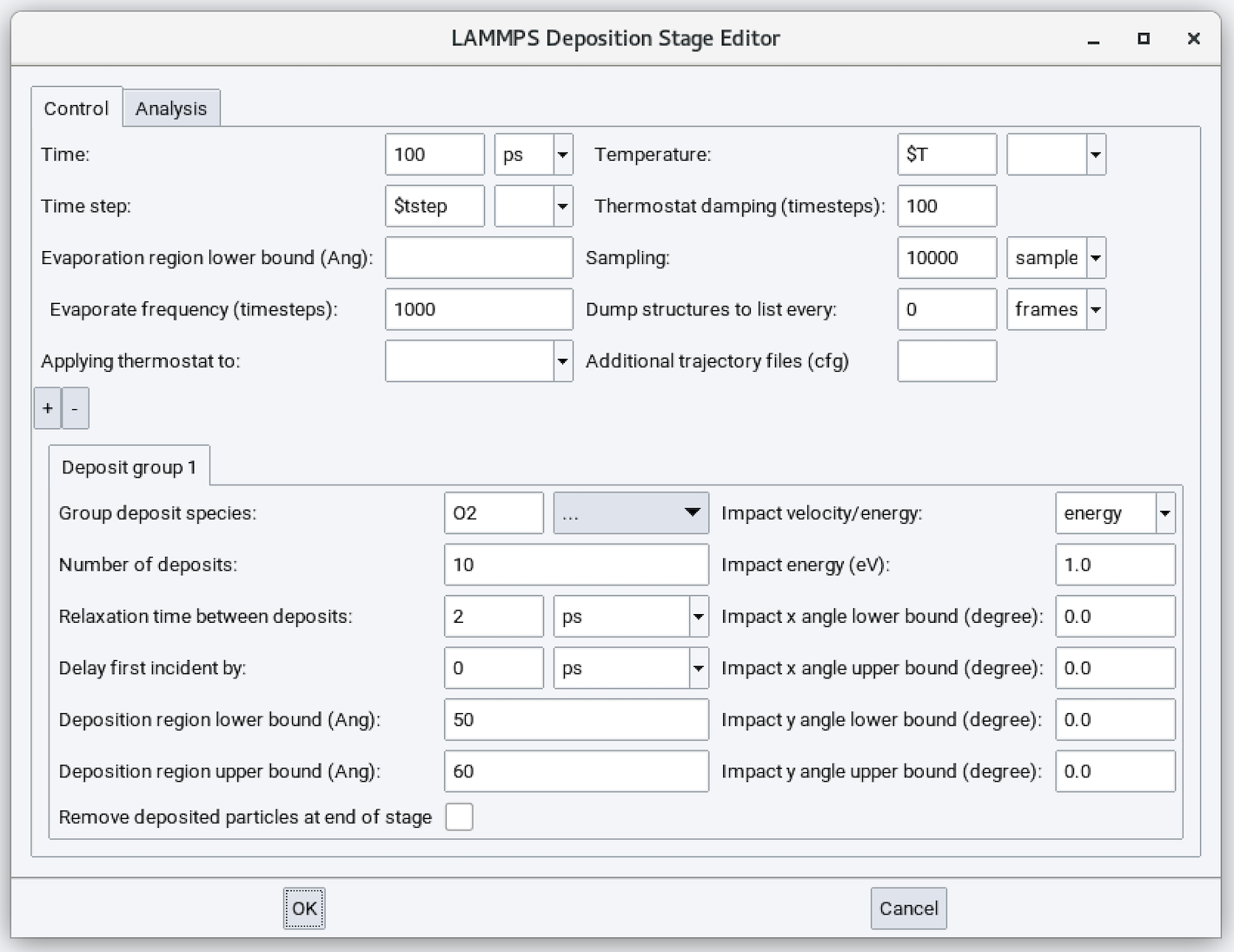
Input parameters are:
- Time: Duration of the simulation run (defaults to 100 ps). The appropriate value for this parameter depends on the Number of deposits, N and Relaxation time between deposits, t. Usually \({T = N * t + C}\) where C is additional several ps to allow all deposits to equilibrate.
- Time step: Time step size employed in solving equations of motion under an NVE ensemble.
- Evaporation region lower bound (Ang): Can be added to remove atoms, molecules, and/or fragments
leaving the surface so they do not accumulate at the upper boundary or re-enter the periodic
boundary condition and deposit on the bottom surface. Usually 5-10 \({\mathring{\mathrm{A}}}\) smaller than box size.
- Evaporation frequency (timesteps): Detect if there are any atoms in the evaporation region every this many steps. Usually 100-1000 is a good number. The default is 1000 steps. Not used if the above option is blank.
- Applying thermostat to: Add Langevin thermostat to a pre-defined subset of atoms. Usually, the
subset region comprises several layers to several 10s of layers of atoms in the middle section
of the slab. This can regulate overall system temperature but does not affect dynamics at the
surface.
- Temperature: Langevin thermostat temperature. Not used if the above option is blank.
- Thermostat damping (timesteps): Langevin thermostat strength. Smaller value means stronger thermostat. Usually 100 time steps are sufficient for a good strength.
- Sampling: Number of samples employed in performing averaging. This parameter does not affect dynamics.
- Dump structures to list every: Together with Time, determines the number of trajectory frames saved to a structure list during the molecular dynamics calculation. This parameter does not affect dynamics.
- Additional trajectory files (cfg): Write additional trajectory files in AtomEye viewer’s cfg format.
The bottom panel controls each of the deposit groups. Use the + / - buttons to add or remove a deposit group.
- Group deposit species: Name of the pre-defined depositing subset.
- Number of deposits: Deposit this many atoms/molecules onto the surface for the entire simulation.
- Relaxation time between deposits: Time interval between deposition events.
- Delay first incident by: Can be used to delay deposition events so if you have multiple depositing groups you can alternate deposition events.
- Deposition region lower bound (Ang): Lower bound of the region to insert new depositing species.
- Deposition region upper bound (Ang): Upper bound of the region to insert new depositing species. New depositing species are inserted randomly within the lower and upper bounds.
- Impact velocity/energy: A drop-down menu to choose between impact energy (eV) or impact velocity (m/s).
- Impact x angle lower bound (degree): Add -X velocity to depositing species.
- Impact y angle upper bound (degree): Add +X velocity to depositing species.
- Impact x angle lower bound (degree): Add -Y velocity to depositing species.
- Impact y angle upper bound (degree): Add +Y velocity to depositing species. These X/Y angle lower/upper bounds allow angled deposition events.
- Remove deposited particles at end of stage: Useful if you want to more closely examine the surface without depositing species.
2.29.5. Distribution Analysis
Distribution analysis is available in the second tab of the Deposition stage:
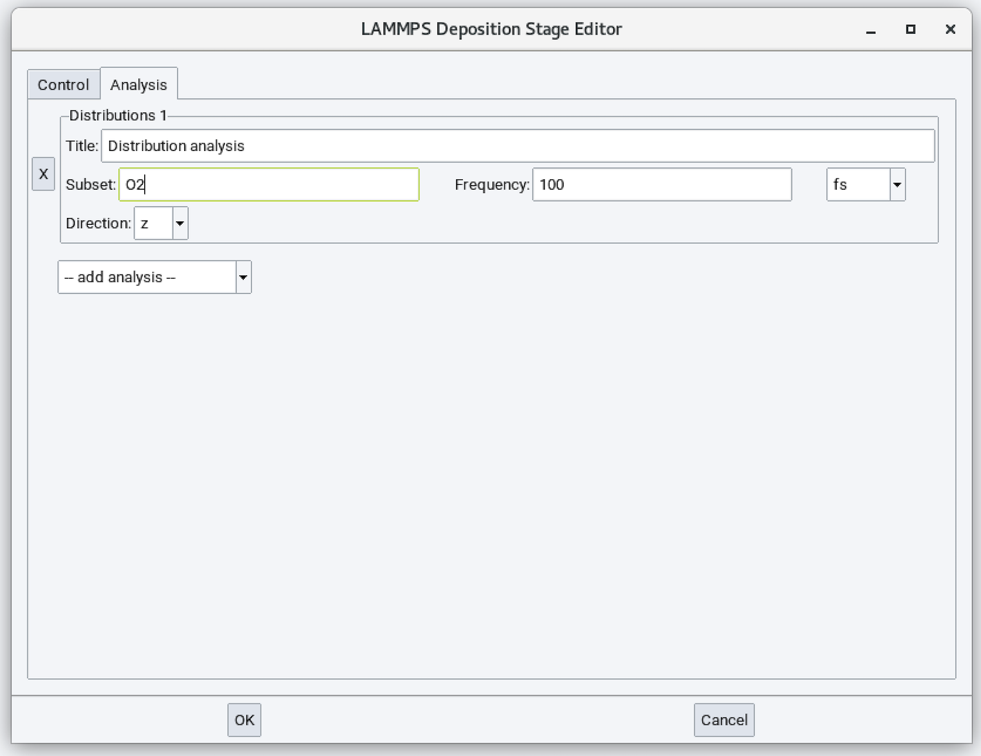
Input parameters are:
- Title: Title of the distribution analysis output.
- Subset: Name of the pre-defined depositing subset to be analyzed.
- Frequency: Frequency of performing statistics. Usually 1/10 of Relaxation time between deposits is a good number.
- Direction: Plot distribution along this direction. Default is Z.
Example output:
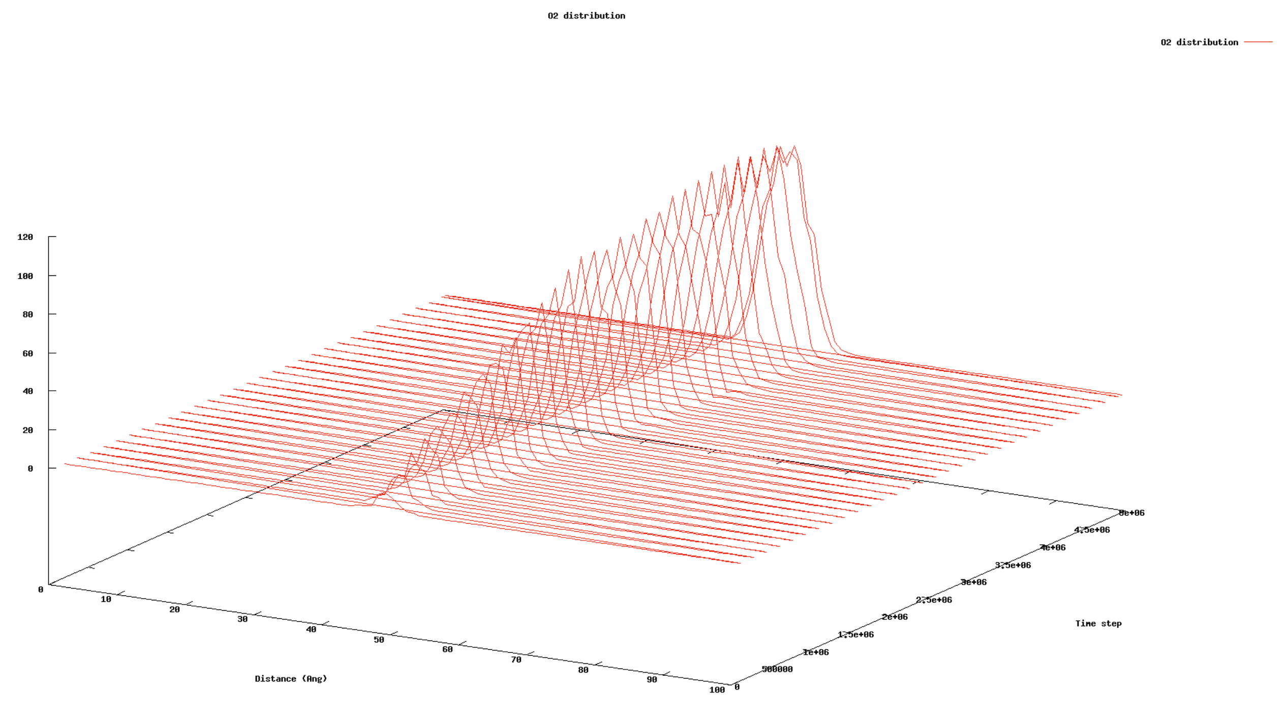
- Vertical axis: Number of deposited species.
- Horizontal axis: Distance (or height) along the defined direction.
- Depth axis: Simulation time step.
| download: | pdf |
|---|