3.10. Electronic Transport

download:pdf

In the present section, we turn to the calculation of several transport coefficients, namely, the electrical conductivity \(\sigma\), the thermopower or Seebeck coefficient \(S\), and the thermal conductivity \(\kappa\). These quantities enter the relations between the electric field \(E\), the temperature gradient \(\nabla T\), and the corresponding electrical and heat currents \(\dot{J_{e}}\) and \(\dot{J_{Q}}\), respectively, which read as [1]

(1)\[\dot{J}_{e,\sigma} = \sigma_{\sigma}E - \sigma_{\sigma}S_{\sigma} \nabla T\]

(2)\[\dot{J}_{Q,\sigma} = T \sigma_{\sigma} S_{\sigma} E - \kappa_{0,\sigma} \nabla T\]

Here, we have already noted the spin-dependent formulation, as we will do throughout this section. The respective spin-independent quantities are arrived at by summing over both spin channels. In general, the transport coefficients are tensors. In addition to \(\kappa_{0,\sigma}\), which is the thermal conductivity at zero electric field, we define the quantity \(\kappa_{electronic,\sigma}\) which is the thermal conductivity at zero electrical current and which is the quantity usually measured. \(\kappa_{electronic,\sigma}\) is generally called the electronic thermal conductivity. According to (1) and (1) both thermal conductivities are related via

(3)\[\kappa_{electronic,\sigma} = \kappa_{0,\sigma} - T \sigma_{\sigma}S_{\sigma}^{2}\]

Finally, we arrive at the total thermal conductivity by adding electronic contribution \(\kappa_{electronic,\sigma}\) and lattice contribution \(\kappa_{lattice}\).

In thermoelectrics, a combination of the above-mentioned transport coefficients gives rise to the so-called figure of merit [2], [3]

\[Z_{\sigma} = \dfrac{\sigma_{\sigma}S_{\sigma}^{2}}{\kappa_{electronic,\sigma} + \kappa_{lattice}}\]

where the product \(\sigma_{\sigma}S_{\sigma}^{2}\) is usually designated as the power factor.

In practice, evaluation of the above-mentioned transport coefficients can be achieved by applying Boltzmann theory [4], [5], [6] Within the framework of this theory the energy-dependent electrical conductivity tensor can be expressed as [7]

(4)\[\sigma_{\alpha \beta, \sigma}(E) = \dfrac{e^{2}}{\Omega_{C}} \sum_{k} \sum_{n} - \dfrac{\partial f(E)}{\partial E} V_{kn\sigma}^{\alpha} V_{kn\sigma}^{\beta} \tau_{kn\sigma}\]

where \(f(E)\) is the Fermi function

\[f(E) = \dfrac{1}{e^{\beta (E-\mu)} + 1}\]

with \(\mu\) being the chemical potential and \(\beta = \dfrac{1}{k_{B}T}\) as usual. In (4), \(\tau_{kn\sigma}\) denotes the relaxation time, which mimics the effects of, e.g., electron Phonon scattering on the electronic states and, in principle, depends on the band index, spin, and k-point. The relaxation time will be addressed in more detail below. Furthermore, \(\nu_{kn\sigma}^{\alpha}\) is the Cartesian component of the group velocity for each band, spin, and k-point, which is given by the first derivative of the band energy with respect to the corresponding Cartesian component of the k-vector as

\[v_{kn\sigma}^{\alpha} = \dfrac{1}{\hbar} \dfrac{\partial \epsilon_{kn\sigma}}{\partial k_{\alpha}}\]

Defining, in addition, the inverse effective mass tensor in terms of the second derivative of the band energies with respect to the Cartesian components of the k-vector as

\[\left( \dfrac{1}{m_{n\sigma}^{ * }} \right) = \dfrac{1}{\hbar} \dfrac{\partial ^{2} \epsilon_{kn\sigma}}{\hbar \partial k_{\alpha}\partial k_{\beta}}\]

and, using the Levi-Civita tensor, \(\epsilon_{\alpha \beta \gamma}\), we are furthermore able to write down the energy-dependent Hall conductivity [7] [8]

\[\sigma_{H,\alpha \beta \gamma, \sigma}(E) = \dfrac{e^{3}}{\Omega_{c}} \sum_{k} \sum_{n} - \dfrac{\partial f(E)}{\partial E} \sigma_{\mu \nu} v_{kn \sigma}^{\alpha} \left( \dfrac{1}{m_{n\sigma}^{*}(k)} \right) _{\beta \mu} v_{kn\sigma}^{\nu} \epsilon_{\mu \nu \gamma} \tau_{kn \sigma}^{2}\]

which will enter the calculation of the Hall coefficient below.

In passing, we mention that the expressions for the group velocity and the inverse effective mass tensor may still be rewritten using \(k \cdot p\) perturbation theory in terms of the momentum operator [9].

The calculation of the electrical conductivity and the related transport properties can be much simplified by defining the so-called transport distribution [2] [3]

(5)\[\Xi_{\alpha \beta, sigma} = \dfrac{1}{\Omega_{c}} \sum_{k} \sum_{n} v_{kn\sigma}^{\alpha} v_{kn\sigma}^{\beta} \tau_{kn\sigma} \delta (E - \epsilon_{kn \sigma})\]

Note that the transport distribution is symmetric with respect to exchange of the Cartesian components. With the help of the previous definition, we can write the transport coefficients as

(6)\[\sigma_{\alpha \beta, \sigma} = e^{2} \int_{-\infty}^{\infty} dE \left( - \dfrac{\partial f(E)}{\partial E} \right) \Xi_{\alpha \beta, \sigma} (E)\]

\[\Upsilon_{\alpha \beta, \sigma} = e^{2} \int_{-\infty}^{\infty} dE \left( - \dfrac{\partial f(E)}{\partial E} \right) \Xi_{\alpha \beta, \sigma} (E) (E - \mu)\]

(7)\[\kappa_{\alpha \beta, \sigma} = e^{2} \int_{-\infty}^{\infty} dE \left( - \dfrac{\partial f(E)}{\partial E} \right) \Xi_{\alpha \beta, \sigma} (E) (E - \mu)^{2}\]

While the electrical conductivity is directly given by (5) and the electronic part of the thermal conductivity by (7), the thermopower is obtained from the matrix equation

\[ S_{\alpha \beta, \sigma} = \sum_{\gamma} \left( \sigma_{\sigma}^{-1} \right)_{\alpha \gamma} \Upsilon_{\gamma \beta, \sigma}\]

The negative derivative of the Fermi function with respect to energy is

\[- \dfrac{\partial f(E)}{\partial E} = \beta \dfrac{e^{\beta (E - \mu)}}{\left( e^{\beta (E - \mu)} +1 \right)^{2}}\]

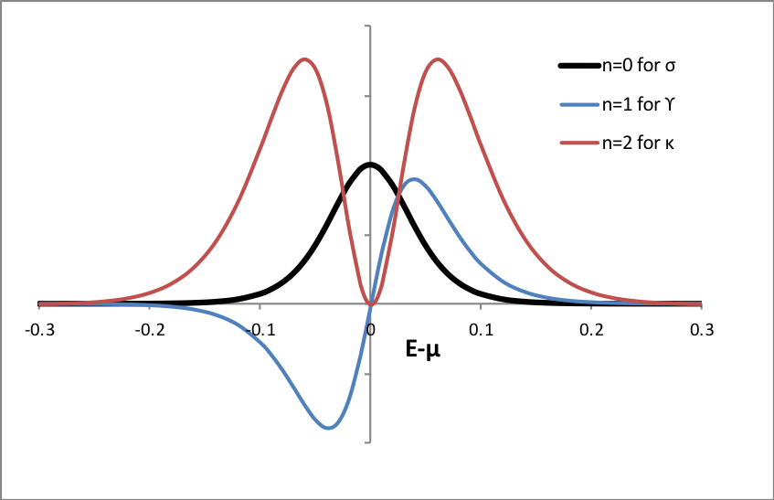
In equations (6) to (7) the effective integration range around the Fermi level (chemical potential) is determined by \(- \frac{\partial f(E)}{\partial E} \left( \beta (E-\mu) \right)^{n} = - \frac{e^{\beta (E-\mu)}}{\left( e^{\beta (E-\mu)} + 1 \right)^{2} \left( \beta (E-mu) \right)^{n}}\). These functions are plotted below for \(n=0,1,2\). Obviously, this restricts the energy integration to a narrow range around the Fermi energy. However, at elevated temperatures, this energy range may be large enough to smear out rather fine details of the electronic structure.

In close analogy to the transport distribution, we define the so-called Hall distribution by

\[\Theta_{H, \alpha \beta \gamma, \sigma} (E) = \dfrac{1}{\Omega_{c}} \sum_{k} \sum_{n} \sum_{\mu \nu} v_{kn\sigma}^{\alpha} \left( \dfrac{1}{m_{n\sigma}^{*}(k)} \right) _{\beta \mu} v_{kn\sigma}^{\nu} \epsilon_{\mu \nu \gamma} \tau_{kn\sigma}^{2} \delta (E-\epsilon_{kn\sigma})\]

from which the Hall conductivity is calculated as

\[\sigma_{H, \alpha \beta \gamma} = e^{3} \int_{-\infty}^{\infty} dE \left( - \dfrac{\partial f(E)}{\partial E} \right) \Theta_{H, \alpha \beta \gamma, \sigma} (E)\]

Finally, the Hall conductivity in combination with the electrical conductivity gives rise to the Hall coefficient [10] [11]

\[R_{H, \alpha \beta \gamma, \sigma} = \dfrac{E_{\beta}^{ind}}{\dot{J}_{e,\alpha}^{appl}B_{\gamma}^{appl}} = \sum_{\mu \nu} \left( \sigma_{\sigma}^{-1} \right)_{\alpha \mu} \sigma_{H, \mu \nu \gamma, \sigma} \left( \sigma_{\sigma}^{-1} \right)_{\nu \beta}\]

Note that all the just calculated transport coefficients can be completely accessed from the electronic structure were it not for the relaxation time \(\tau_{kn\sigma}\). However, detailed studies have shown that the relaxation time, to a good approximation, is isotropic [11]. For this reason, we follow the usual treatment and keep the relaxation time constant, in which case it cancels completely from both the thermopower and the Hall coefficient.

The effective mass tensor mentioned above has received a lot of interest, especially in the semiconductor industry. From a semiclassical point of view, it influences the response of the electrons to an external electric or magnetic field and, hence, the carrier mobility. It thereby directly affects the transport properties of a material, which have a strong impact on the properties of semiconductor devices. In general, the effective mass of the charge carriers is a genuine fingerprint of the materials properties. While in semiconductors effective masses usually are of the order of 1 electron mass but may well be one or even two orders of magnitude smaller or larger, extremely high effective masses of the order of 1000 electron masses have been observed in the heavy fermion systems, where the strong coupling of the conduction electrons to the well localized f electrons leads to the strongly enhanced mass renormalization.

The definition and calculation of the effective mass from the electronic band structure is, of course, predicated on the isotropic and parabolic dispersion relation of free electrons

\[\epsilon_{k} = \dfrac{\hbar^{2}}{2m} k^{2}\]

with \(m\) being the bare electron mass. Obviously, the latter is given as the second derivative or equivalently the curvature of the band. These basic relations can be readily generalized to realistic band structures by defining the effective mass tensor as defined already above as the second derivative of the \(\epsilon_{kn\sigma}\) with respect to the components of the k-vector.

Ashcroft and Mermin, while restricting their considerations to k-space regions near the band extrema, use the same definition with a - and + sign appended for band maxima and minima, respectively [9].

This reflects the main interest from semiconductor physics, where partially filled bands, which are accessible to charge carrier transport induced by external fields, develop only at non-zero temperature and by doping. They thus affect only the electronic states near the valence band maximum and conduction band minimum. Near to these band extrema, knowledge of the effective mass tensor gives access to an effective square-root like density of states, which is renormalized by the ratio of the bare and effective masses and determines the distribution of excited carriers at elevated temperatures and under doping.

While the effective mass tensor in principle can be determined, via the effective mass theorem growing out of \(k \cdot p\) perturbation theory, from the momentum operator, we prefer to determine the effective mass tensor directly from the knowledge of the electronic states \(\epsilon_{kn\sigma}\) and a subsequent least-squares fit to these states. Such a procedure is implemented in MedeA. To be specific, a least-squares fit routine of up to fourth-order has been implemented, which allows you to obtain the effective mass tensor from the electronic states \(e_{kns}\) on a very fine grid of k-points centered about the point of interest. In practice, a grid spacing of 5 x 10^-4 \({\mathring{\mathrm{A}}}\)^-1 is a good choice.

[1]	Gerd Czycholl, Theoretische Festk\({\ddot{o}}\) rperphysik, Rd.Springer.com, (Berlin, Heidelberg: Springer Berlin Heidelberg, 2008).

[2]	(1, 2) G D Mahan and J O Sofo, “The Best Thermoelectric,” Proceedings of the National Academy of Sciences 93, no. 15 (July 23, 1996): 7436-7436.

[3]	(1, 2) T Scheidemantel, C Ambrosch-Draxl, T Thonhauser, J Badding, and J Sofo, “Transport Coefficients From First-Principles Calculations,” Physical Review B 68, no. 12 (September 2003): 125210.

[4]	B R Nag, Electron Transport in Compound Semiconductors, vol. 11, (Springer, 1980).

[5]	Philip B Allen, “Boltzmann Theory and Resistivity of Metals,” in Quantum Theory of Real Materials, ed. by J Chelikowsky and Steven G Louie, (Springer, 1996).

[6]	J M Ziman, Electrons and Phonons: The Theory of Transport Phenomena in Solids, (Oxford University Press, USA, 2001).

[7]	(1, 2) Georg K H Madsen and David J Singh, “BoltzTraP. a Code for Calculating Band-Structure Dependent Quantities,” Computer Physics Communications 175, no. 1 (July 2006): 67-71.

[8]	Werner Schulz, Philip B Allen, and Nandini Trivedi, “Hall Coefficient of Cubic Metals,” Physical Review B 45, no. 19 (May 1992): 10886-10890.

[9]	(1, 2) NW Ashcroft and ND Mermin, Solid State Physics, Holt-Saunders, 1976.

[10]	Georg K H Madsen and David J Singh, “BoltzTraP. a Code for Calculating Band-Structure Dependent Quantities,” Computer Physics Communications 175, no. 1 (July 2006): 67-71.

[11]	(1, 2) Werner Schulz, Philip B Allen, and Nandini Trivedi, “Hall Coefficient of Cubic Metals,” Physical Review B 45, no. 19 (May 1992): 10886-10890.

download:pdf