2.6. Flowcharts
Contents
| download: | pdf |
|---|
The MedeA environment provides graphical flowcharts to support the efficient construction of complex computational protocols. These flowcharts can be easily created to describe and control the flow of calculations, allowing simple and straightforward access to MedeA’s various computation engines, such as LAMMPS, GIBBS, VASP, MOPAC and Gaussian. These different engines may be combined within a single flowchart, so that a VASP optimization of a unit cell, for example, may be employed as a prelude to a larger scale LAMMPS simulation using an embedded atom method forcefield. In addition, the structure can be modified within the flowchart using the provided building and editing capabilities.
The backbone of the flowchart infrastructure is the Tcl language (see https://www.tcl.tk/) which can be directly accessed within custom-scripting stages. Once created the flowcharts can be saved as ASCII files allowing them to be reused and distributed.
Although flowcharts are customizable and flexible their use is straightforward. In this section the basic concepts are summarized, allowing for the construction of both simple and complex flowcharts. Additional details for specific tools are provided elsewhere within the MedeA User’s Guide.
2.6.1. Flowcharts Overview
Flowcharts are accessed via the Job Control >> New Job… menu item. This command yields the main flowchart user interface, where flowcharts are constructed, read from disk or from previous calculations, or saved to the disk.
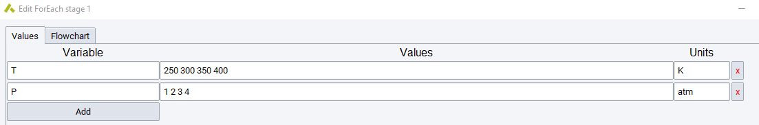
Flowcharts provide a variety of control capabilities, such as a While Loop, For Loop, Foreach Structure Loop, If and Foreach Loop. This allows for considerable flexibility in the automation of simulations. For example, a scan of possible system temperatures and pressures for molecular dynamics calculations may be achieved with nested Foreach loops.
Additionally, custom Tcl scripting may be included in a flowchart. Key results from simulation stages are available as variables, which can be operated on, tabulated, and also used to control subsequent stages, allowing the convenient construction of highly automated procedures for selected applications. If more complex manipulation of the results are required, a custom Tcl stage can be used to process the outputs of the current and any previous stages.
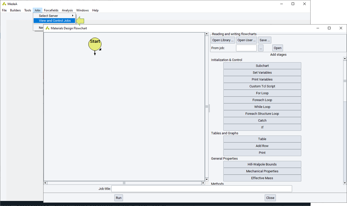
Materials Design flowcharts begin with the Start command which is automatically placed on the left-hand pane of the flowchart dialog. Typically, after initiating a flowchart with a Start stage, a number of variables will be set using a Set Variables stage. The stage is added to the flowchart by clicking the Set Variables button on the right-hand pane.
In general, stages are added to a flowchart by clicking the appropriate element on the right-hand pane of the flowchart dialog or user interface. Once added to a flowchart, most stages may be edited by either right-clicking that element and selecting Edit, or double-clicking on that stage.
A summary of the functionality and use of specific flowchart elements is provided below.
2.6.2. Initialization and Control
This section of the flowchart interface provides the following stages: Start, Subchart, Set Variables, Print Variables, Custom Tcl Script, and loop related commands: For Loop, Foreach Loop, While Loop, Foreach Structure Loop, Catch and If.
As discussed above, every flowchart begins with a Start stage, this is employed as the starting point of execution for the flowchart, and is automatically included in the flowchart. The Subchart stage is simply a container that can hold other flowcharts. This provides a convenient way to break up a large more complicated flowchart into simpler parts and provides a simple way to include a previous flowchart as a building block into a more complicated protocol.
The Set Variables stage allows the user to set the value and units of specific variables that will be employed in later stages in the flowchart. For example, the Set Variables stage can be used to set:
| Variable | Value | Units |
| T | 300 | K |
| tstep | 1 | fs |
| P | 1 | atm |
These variables will then be used throughout subsequent stages in LAMMPS
calculations, which employ T, tstep, and P as default variables for
temperature, timestep, and pressure respectively. This centralization of
the variable setting is convenient in exploring the effect of the system
variables on simulated properties.
Once declared variables can be accessed, in accordance to the Tcl paradigm,
by adding a $ sign in front of the variable name, for example, the variable tstep can
be accessed with $tstep.
The Print Variables reports (calculated) variables matching a specific name, including variables created and made accessible by any previous stage. These variables can be printed to tables or added to structure lists.
The Custom Tcl Script allows you to enter, or retrieve from a file Tcl commands (see https://www.tcl.tk/) which may be used to carry out specific actions during the execution of a flowchart. This can be useful in preparing result summaries or in determining whether specific simulation conditions have been met.
The For Loop includes a flowchart executed repeatedly as defined by the control variables and test conditions.
The Foreach Loop and While Loop stages allow for the
introduction of control structures within a flowchart. In each case,
allowing for the introduction of a complete flowchart to be executed
repeatedly until the foreach vector (like {T,P}) of variables is
exhausted, or the while condition is no longer true.
The Foreach Structure Loop takes structures contained in a Structures List or a previous Trajectory and performs on each of these structures the same calculation protocol as defined in the Foreach Structure Loop flowchart.
The loops are either synchronous, meaning that each iteration is completed before the next is started, or asynchronous, where multiple iterations run in parallel. Asynchronous operation mode is switched on by checking Run the different loop iterations simultaneously, specifying the degree of parallel operation by the parameter Maximum number of jobs to submit simultaneously. All looping structures have an option to Catch and ignore errors in the iterations.
The Catch stage allows for more elaborate error handling, that is in case the flowchart runs into an error, it is caught and another flowchart executed.
The If stage allows execution of a flowchart, if a condition is true (then), or an alternative flowchart (else).
2.6.3. Tables and Graphs
This section allows do define a Table, insert results as soon as they occur with Add Row and finally Print the entire table. The flowchart below is just an illustration, leaving out all looping and calculation.
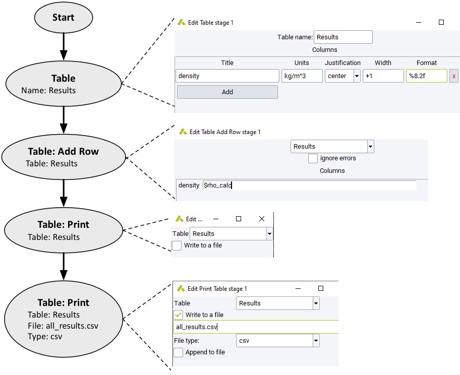
With Table you define a Table by giving it a name and adding columns. Each column has a
Title:Name of the column
Units: Results are converted into units chosen. If no unit is specified, the default unit is used.
Justification: Left, right, or center
Width: How much “space” on the left and right
Format: Can be provided in the printf format. For example;%dor%ifor integer values,%ffor float/double values,%cfor characters,%sfor strings, and%xfor hexadecimal values.Hint
The maximum number of characters/digits that can be used to print a given variable can be defined by an integer value between the
%sign and the character. In case of a float value two numbers, separated by a comma, can be used. In this case the second number defines the number of digits after the comma used to print the value. For example,%8.2fdisplays a floating point variable with up to 8 characters in total and two digits after the comma.
Table: Add Row adds a line of results to a specified table. Variables can be added, in accordance with the Tcl paradigm,
by adding a $ sign in front of the variables name, e.g., the variable Etotal_calc can
be printed with $Etotal_calc into a table.
Table: Print the selected Table. You can also save or
append the result to a file as formatted text,
comma separated values (csv), tab-delimited, or
delimited by a different Separator like ;.
2.6.4. General Properties
Mechanical Properties determines the mechanical properties with LAMMPS or VASP based on given Strains. For more information refer to the chapter on the Theory of elasticity.
Hill-Wallpole bounds: applies Hill-Walpole statistics on top of Mechanical Properties (see the section on Hill-Walpole bounds for amorphous systems).
Effective Mass: uses VASP to determine the effective mass for a specified k-point. For a more detailed description of the use of this stage see the section on Accurate Effective Mass calculations.
2.6.5. Methods
The Methods section of the flowchart interface provides access to a computational engine such as GIBBS, LAMMPS, MOPAC, GAUSSIAN or VASP (VASP flowcharts or a stage accessing the VASP GUI otherwise accessible from the Tools menu). In each case, the interface provided allows you to start a new flowchart, and execute relevant specific commands within this new flowchart.
In addition, there are methods available making use of the computational engines above to calculate vibrational properties (Phonon), to optimize cluster expansions for alloy and other disordered systems and perform Monte Carlo simulations for larger ensembles (UNCLE), to predict properties of polymers using correlations (P3C) or group contributions (QSPR), and to optimize force field parameters by fitting to ab-initio data (FFO).
Additional information on each of the Methods available in this section of the flowchart interface is available in the section of the User’s Guide dealing with each method.
2.6.6. Building and Editing
Flowchart building commands allow for the construction and adjustment of atomic models.
2.6.6.1. Set Cell
The Set Cell stage permits the adjustment of unit cell dimensions for periodic systems. Here a variety of options are supported, the density or volume may be specified, or an expansion factor applied to the current system, or specific unit cell dimensions set. This stage may be combined with an appropriate Foreach Loop to explore the volumetric or density specific behavior of a given system property.
2.6.6.2. Change periodicity
A stage to turn on or remove periodic boundary conditions. In this stage the specify a gap to leave between the periodic building blocks. This stage may be used to combine a non periodic calculation, for example with MOPAC, with a periodic VASP calculation.
2.6.6.3. Supercell
The Supercell command may be applied to increase the size of a given model. As this building process is executed on the JobServer this is an efficient mechanism to create large systems.
2.6.6.4. Amorphous builder
The Amorphous Builder stage can be used to create amorphous models. System composition source can be set to the current system, where the current structure is split into molecules and recombined, to composition files saved on the local machine, and to a composition used in a previous job with jobserver. The system geometry of the amorphous material can be either bulk cell or layer and is build according to the set Temperature and cell dimensions. The later is set with specify cell and can be a mixture of the specific cell dimensions a, b, and c in combination with density. Accordingly additional options become available. The number of mols of the defined composition is set with Nmols. As this is a stochastic process the number of configurations that are to be created can be set. Multiple amorphous structures can be used to determine the average property of a given model. See the chapter on Amorphous Materials Builder for more information.
2.6.6.5. Thermoset Builder
The Thermoset Builder creates a densely crosslinked thermoset structure from an equilibrated bulk amorphous system. The crosslinking process involves the creation of bonds between user specified sets of atoms (sites), achieved in a series of crosslinking cycles through the growth of a capture sphere about each site.
During each cycle, bonds are created between reacting pairs of atoms lying within each site’s capture sphere until the maximum allowed number of connections specified for each site has been reached. After cleaning to remove high energy interactions, each cycle is completed by performing structural relaxation using a small number of iterations of molecular dynamics followed by minimization.
The process continues through the growth of the capture sphere until either a maximum realistic radius has been reached, or until other specified conditions prevail (exceeding a maximum number of cycles, the maximum extent of reaction, threshold strain energy in the system, or detection of catenations between small rings).
Note that the Thermoset Builder operates on a principle analogous to that of the Polymer Builder. Thus, whereas the Polymer Builder operates by connecting together polymer repeat units rather than monomers (e.g. -(CH 2-CH 2)- rather than H 2C=CH 2for polyethylene), the Thermoset Builder creates crosslinks in a pre-cured system of network fragments (e.g. H 2N-R-NH 2and H 3C-CH(OH)- CH 2-O-R’-O-CH 2-CH(OH)-CH 3for an epoxy resin system, where the terminal nitrogens of the amine are sites capable of making up to two connections and the terminal carbons of the diglycidyl ether fragment are sites each capable of reacting once).
Note
The extent of reaction of a given site type is the total number of crosslinks formed at/by sites of that type (e.g. type ‘A’), divided by the total number of crosslinks possible at those sites, with the latter being equal to the product of the total number of sites of a given type and the maximum number of bonds that can be created at the site defined by, for example, Site A max reactions.
Whenever the Maximum extent of reaction criterion is exceeded at the end of a crosslinking cycle, the builder will stop. Moreover, if the crosslinked system is stoichiometrically unbalanced, the criterion applies to sites of the component present in excess.
2.6.6.6. Parameters
Required input parameters are as follows:
Number of crosslink site types: A value of 1 would be used to mimic self-crosslinking (e.g. as produced by irradiation), while more commonly a value of 2 would be used to simulate reactions such as those involved in epoxy resin curing.
Site A subset: MedeA subset name for a set of crosslinkable sites.
Site A max reactions: number of new bonds between sites of type A and other sites. Note that after adding each new bond, a hydrogen atom is removed from the site A atom.
Site A substitution effect prob: Whenever the site can participate in more than a single crosslinking reaction, this list of parameters can be used to control the relative probability of successive reactions at the site. For example, a site capable of participating in two reactions (such as an amine first transformed from primary to secondary, and then from secondary to tertiary) may utilize this parameter to specify the relative probability of crosslink formation at sites which have reacted once already relative to those which have never reacted. By extension, relative reaction probabilities at a site capable of participating in N reactions would be specified by giving a list of (N-1) probabilities, which will often take the form of a list of decreasing values. Note that for common amine-cured epoxy thermosets, the relative rates of secondary and primary amine reactions may often lie in the range 0.2-0.6 for aromatic amines, with larger values for aliphatic amines (see, for example, “Cross-linking of Epoxy Resins”, K. Dusek, in Rubber-modified thermoset resins ACS Adv. Chem. Ser. vol 208 (1984)).
Site B subset: second subset when two site types have been specified.
Site B max reactions: maximum number of connections to a type B site.
Site B substitution effect prob: See explanation of the analogous parameter for sites of type A.
Allowed reactions: between the two types of sites, only displayed when more than one site type is used. Most commonly this will only be between the different types of site.
Beginning capture radius; in Angstroms applied at the start of the crosslinking process.
Capture radius increment: capture sphere radius is increased when no bondable pairs are found to lie within the current sphere for all sites.
Relaxation conditions: Indicates whether the relaxation dynamics applied at the end of each cycle are to be performed under constant volume (NVT) or constant pressure (NPT) conditions.
Relaxation iterations (per cycle): sets the total amount of structural relaxations.
Note
The use of a large value (>10) will significantly increase the time taken to perform the crosslinking, and is best used for very rigid systems.
Maximum extent of reaction: is the fraction of the maximum possible reactions reached, at which the building will stop.
Maximum capture radius: capture radius at which the building will stop.
Maximum crosslinking cycles: reduce the number of cycles below that implicitly defined by the maximum, beginning and capture radius increment.
Stop at gelation: Selecting this option will cause the building to terminate immediately after the formation of a 3-dimensional infinite network has been detected, overriding other termination parameters such as the Maximum extent of reaction. This can be useful for studying the gel point itself, and for examining the properties of the network immediately after formation.
Reset Forcefield atom types: this checkbox is selected by default and indicates that forcefield atom types and partial charges will be reassigned following completion of the building, which will often be necessary prior to performing further LAMMPS simulations due to changes in the bonded environment of individual atoms resulting from crosslink formation. Uncheck the option if you wish to exercise complete control over atom types and partial charges.
Write structure after each cycle: If this checkbox is selected, the coordinates and topology of the relaxed structure at the end of each crosslink cycle will be saved in a MedeA trajectory file for later visualization or further manipulation.
Control intramolecular ring formation: Enabling this option can be useful for studying how intramolecular reactions influence network structure and properties such as the gel point or behavior such as elastic constants and thermal conductivity of the final network.
Minimum ring size (atoms): This parameter is only required when limiting intramolecular ring formation is to be applied. Typically, rings containing a small number of atoms are most likely to be formed (where allowable sizes are determined by the bonding topology of the reactants). Consequently, specifying a value equal to ‘n+1’, where ‘n’ denotes the number of atoms in the smallest ring, will exclude only those rings form the network. Conversely, specifying a large value will practically eliminate all intramolecular cycles.
2.6.6.6.1. Properties
This stage generates building related information, including maximum
bond strain, and dimensionality of the structure as a function of
progress of the crosslinking (see Progress.txt and bondEnergy.png on the
Job’s page). A dimensionality of 3 denotes that the gel point has been
exceeded and that a true 3-Dimensional network has been created.
Note
Restarting crosslinking from a partially crosslinked system is not yet supported.
2.6.6.7. Translate Atoms
The Translate Atoms command can be used to adjust the position of atoms within the current system. Thereby it is possible to explicitly select atoms of the active structure or to select a subset. Atoms can be translated by a translation vector or to a point. The displacement can be in fractional or cartesian coordinates.
2.6.6.8. Docking
The Docking stage combines two structures. The host structure is the ‘stream’ structure upon which the Flowchart is operating. The Guest from Job is specified as the final.sci of the specified job on the current Job Server, the Host is specified as the input structure submitted with the flowchart. Number of guests defines how many guest molecules are put into the host, for each guest this process is repeated for Maximum iterations. The Maximum displacement (Ang) should be larger than the diameter of any ring to avoid interlocking of molecules. Scale rotations by and Temperature (K) as well as the underlying theory is explained in the section on Docking.
2.6.6.9. Randomly Substitute Atoms
Replaces a defined number of atoms, accounting for the symmetry of the structure, of element A with either vacancies or atoms of element B. For more information refer to the section on Random Substitution.
2.6.6.10. Simple Dynamics & Minimization
This stage uses the same simple dynamics and minimization algorithm that is also accessible from the MedeA GUI. The Number of dynamics steps and the Number of minimization steps can be set separately. Use this stage to pre-optimize a structure before applying a computationally more demanding algorithm to it.
2.6.6.11. Subset Manager
Manipulate existing subsets in a structure.
2.6.7. Structures Lists
These are a collection of commands to handle Structures Lists:
New List creates a new structure list that is accessible by the current flowchart. The List name and the File name of the structure lists can be defined. If no subfolder is specified the list will be placed in the job folder. The list can be initialized from an initial list that is saved locally on the machine running the MedeA GUI. Note, that multiple structure list can be active at the same time.
Save to List adds the current structure to any of the active structure lists. In addition, the structure can be saved with multiple properties.
Extract from List will extract a structure, specified by Structure index and Configuration index, from any of the active lists.
Sort List will sort any of the active structure lists according to a specific property.
Remove Duplicates from List remove all duplicates from a given list. Duplicates are identified by making use of symmetry.
Compute Descriptors on a list define and compute descriptors on a list.
Apply QSAR model on List by loading the equation from a XML QSAR model file.
2.6.8. Forcefield
Set Forcefield allows you to specify a forcefield.
Assign Atom Types and Charges allows you to readjust or set atomic forcefield parameters. This requires a forcefield with auto-typing.
Note
When using a custom forcefield in conjunction with a remote JobServer it is
required that the forcefield is placed in the identical directory on the JobServer.
To facilitate this, it is recommended to place the custom forcefield in a directory named Forcefields/custom located in Linux
under {/home/username}/MD/2.0/data. On Windows save it to C:/MD/2.0/data/Forcefields/custom.
2.6.9. Analysis
Orientation determines the orientation of a subset to a given reference vector:(x, y,:highlightgray:z).
2.6.10. Properties
Below listed properties are made available in the flowchart after a specified stage. To
access any of these use a $ sign in front of the property name. For example, the variable Etotal_calc can
be accessed with $Etotal_calc.
2.6.10.1. MedeA LAMMPS
| Property | Units | averaged |
|---|---|---|
| t_calc | fs | no |
| T_calc | K | yes |
| P_calc | atm | yes |
| V_calc | \({\mathring{\mathrm{A}}}\)3 | yes |
| rho_calc | g/mL | yes |
| Etotal_calc | kcal/mol | yes |
| Epot_calc | kcal/mol | yes |
| Ekin_calc | kcal/mol | yes |
| Evdw_calc | kcal/mol | yes |
| Ecoul_calc | kcal/mol | yes |
| Enonbond_calc | kcal/mol | yes |
| Ebond_calc | kcal/mol | yes |
| EAngle_calc | kcal/mol | yes |
| Edihed_calc | kcal/mol | yes |
| Eimp_cal | kcal/mol | yes |
| Eint_calc | kcal/mol | yes |
| a_calc | \({\mathring{\mathrm{A}}}\) | yes |
| b_calc | \({\mathring{\mathrm{A}}}\) | yes |
| c_calc | \({\mathring{\mathrm{A}}}\) | yes |
| alpha_calc | 0 | yes |
| beta_calc | 0 | yes |
| gamma_calc | 0 | yes |
| Sxx_calc | atm | |
| Syy_calc | atm | yes |
| Szz_calc | atm | yes |
| Syz_calc | atm | yes |
| Sxz_calc | atm | yes |
| Sxy_calc | atm | yes |
| deltaQ_calc. | kcal/mol | no |
| dQ/dt_calc | kcal/mol/fs | yes |
| deltapx_calc | \({\mathring{\mathrm{A}}}\)/fs*g/mol | no |
| dpx/dt_calc | \({\mathring{\mathrm{A}}}\)/fs*g/mol/fs | yes |
| CED_calc | J/cm3 | yes |
| CEDvdw_calc | J/cm3 | yes |
| CEDcoul_cal | J/cm3 | yes |
| dHvap (ideal)_calc | kJ/mol | yes |
| nSteps_calc | no | |
| Fmax_calc | kcal/mol/\({\mathring{\mathrm{A}}}\) | no |
| Frms_calc | kcal/mol/\({\mathring{\mathrm{A}}}\) | no |
| P_calc | atm | no |
| V_calc | \({\mathring{\mathrm{A}}}\)3 | no |
| rho_calc | g/mL | no |
| Sxx_calc | atm | no |
| Syy_calc | atm | no |
| Szz_calc | atm | no |
| Syz_calc | atm | no |
| Sxz_calc | atm | no |
| Sxy_calc | atm | no |
2.6.10.2. MedeA VASP
Different properties are calculated depending on the type of VASP calculation configured within the VASP stage. Properties listed in the first table are always available after a successful VASP calculation.
| Property | Units | Description |
|---|---|---|
| Eelectronic_calc | eV | VASP energy (for primitive cell) |
| Eelectronic_calc | eV | VASP energy (for primitive cell) |
| Eelectronic_conventionalCell_calc | eV | VASP energy (for conventional cell) |
| Eelectronic_empiricalFormula_calc | eV | VASP energy (for empirical formula) |
| Eelectronic_sigma0_calc | eV | VASP energy extrapolated to zero smearing (for primitive cell) |
| Enon-dispersive_calc | eV | VASP energy without van der Waals contribution, if van der Waals forcefield is applied (for primitive cell) |
| EVanderWaals_calc | eV | VASP energy, van der Waals contribution, if van der Waals forcefield is applied (for primitive cell) |
| FormulaPrimitiveCell_calc | Formula of the primitive cell | |
| FormulaConventionalCell_calc | Formula of the conventional cell | |
| FormulaEmpirical_calc | Empirical formula | |
| FactorEmpiricalToPrimitive_calc | Factor to convert empirical formula to primitive cell formula | |
| FactorEmpiricalToConventional_calc | Factor to convert empirical formula to conventional cell formula | |
| Efermi_calc | eV | Fermi energy |
| a_calc | \({\mathring{\mathrm{A}}}\) | Lattice parameter a |
| b_calc | \({\mathring{\mathrm{A}}}\) | Lattice parameter b |
| c_calc | \({\mathring{\mathrm{A}}}\) | Lattice parameter c |
| alpha_calc | degree | Lattice parameter |
| beta_calc | degree | Lattice parameter |
| gamma_calc | degree | Lattice parameter |
| Vprim_calc | \({\mathring{\mathrm{A}}}\)3 | Volume (primitive cell) |
| rho_calc | Mg/m3 | Density |
| mu_calc | \({\mu_B}\) | Total magnetic moment (spin-polarized) |
| mux_calc | \({\mu_B}\) | Total magnetic moment in x direction (spin-orbit or non-collinear magnetic) |
| muy_calc | \({\mu_B}\) | Total magnetic moment in y direction (spin-orbit or non-collinear magnetic) |
| muz_calc | \({\mu_B}\) | Total magnetic moment in z-direction (spin-orbit or non-collinear magnetic) |
| Eformation_calc | kJ/mol | Formation energy |
| Hformation_calc | kJ/mol | Heat of formation |
| approximateMaterial_calc | Type of material: metal, semiconductor or insulator | |
| approximateGap_calc | eV | Band gap width |
| approximateGapType_calc | Type of band gap: direct, indirect, no | |
| approximateVBMaxPosition_calc | Approximate position of the valence band maximum in the Brillouin zone (fractional coordinates of a vector in k-space) | |
| approximateCBMinPosition_calc | Approximate position of the conduction band minimum in the Brillouin zone (fractional coordinates of a vector in k-space) | |
| return_status_calc | Return status: finished, warnings, error | |
| planewaveCutoff_calc | eV | Plane wave cutoff |
| nKPoints_calc | Number of k-points in the Brillouin zone | |
| FFTGridX_calc | Coarse Fast-Fourier grid in x direction | |
| FFTGridY_calc | Coarse Fast-Fourier grid in y direction | |
| FFTGridZ_calc | Coarse Fast-Fourier grid in z direction | |
| FFTFineGridX_calc | Fine Fast-Fourier grid in x direction | |
| FFTFineGridY_calc | Fine Fast-Fourier grid in y direction | |
| FFTFineGridZ_calc | Fine Fast-Fourier grid in z direction | |
| FFTAddedGridX_calc | Extrafine Fast-Fourier grid in x direction added for evaluation of augmentation charges and accurate forces | |
| FFTAddedGridY_calc | Extrafine Fast-Fourier grid in y direction added for evaluation of augmentation charges and accurate forces | |
| FFTAddedGridZ_calc | Extrafine Fast-Fourier grid in z direction added for evaluation of augmentation charges and accurate forces | |
| FFTCompleteGridX_calc | Minimum Fast-Fourier grid in x direction to avoid aliasing errors | |
| FFTCompleteGridY_calc | Minimum Fast-Fourier grid in y direction to avoid aliasing errors | |
| FFTCompleteGridZ_calc | Minimum Fast-Fourier grid in z direction to avoid aliasing errors |
| Property | Units | Description |
|---|---|---|
| V_calc | \({\mathring{\mathrm{A}}}\)3 | Volume (conventional cell) |
| P_calc | GPa | Pressure |
| Sxx_calc | GPa | Stress tensor component xx |
| Syy_calc | GPa | Stress tensor component yy |
| Szz_calc | GPa | Stress tensor component zz |
| Syz_calc | GPa | Stress tensor component yz |
| Sxz_calc | GPa | Stress tensor component xz |
| Sxy_calc | GPa | Stress tensor component xy |
| Property | Units | Description |
|---|---|---|
| Etotal_calc | kJ/mol | Total energy (average) |
| Etotal_uncertainty_calc | kJ/mol | Total energy (standard deviation) |
| Ekin_calc | kJ/mol | Kinetic energy (average) |
| Ekin_uncertainty_cal | kJ/mol | Kinetic energy (standard deviation) |
| Epot_calc | kJ/mol | Potential energy (average) |
| Epot_uncertainty_calc | kJ/mol | Potential energy (standard deviation) |
| V_calc | \({\mathring{\mathrm{A}}}\)3 | Volume (average) |
| V_uncertainty_calc | \({\mathring{\mathrm{A}}}\)3 | Volume (standard deviation) |
| P_calc | GPa | Pressure (average) |
| P_uncertainty_calc | GPa | Pressure (standard deviation) |
| T_calc | K | Temperature (average) |
| T_uncertainty_cal | K | Temperature (standard deviation) |
| Sxx_calc | GPa | Stress tensor component xx (average) |
| Sxx_uncertainty_calc | GPa | Stress tensor component xx (standard deviation) |
| Syy_calc | GPa | Stress tensor component yy (average) |
| Syy_uncertainty_calc | GPa | Stress tensor component yy (standard deviation) |
| Szz_calc | GPa | Stress tensor component zz (average) |
| Szz_uncertainty_calc | GPa | Stress tensor component zz (standard deviation) |
| Syz_calc | GPa | Stress tensor component yz (average) |
| Syz_uncertainty_calc | GPa | Stress tensor component yz (standard deviation) |
| Sxz_calc | GPa | Stress tensor component xz (average) |
| Sxz_uncertainty_calc | GPa | Stress tensor component xz (standard deviation) |
| Sxy_calc | GPa | Stress tensor component xy (average) |
| Sxy_uncertainty_calc | GPa | Stress tensor component xy (standard deviation) |
| Property | Units | Description |
|---|---|---|
| BaderCharges_calc | electron charge. Bader charge per atom for each site | |
| BaderChargeTransfers_calc | electron charge. Charge transfer per atom for each site | |
| BaderVolumes_calc | \({\mathring{\mathrm{A}}}\)3 | Bader volume per atom for each site |
| BaderDistances_calc | \({\mathring{\mathrm{A}}}\) | Bader distance for each site |
| BaderVacuumCharge_calc | electron charge. Bader charge of the vacuum region | |
| BaderVacuumVolume_calc | \({\mathring{\mathrm{A}}}\)3 | Bader volume of the vacuum region |
| BaderTotalVolume_calc | \({\mathring{\mathrm{A}}}\)3 | Total Bader volume |
| Property | Units | Description |
|---|---|---|
| DOS_approximateMaterial_calc | Type of material: metal, semiconductor or insulator | |
| DOS_approximateGap_calc | eV | Band gap width |
| DOS_approximateGapType_calc | Type of band gap: direct, indirect, no | |
| DOS_approximateVBMaxPosition_calc | Approximate position of the valence band maximum in the Brillouin zone (fractional coordinates of a vector in k-space) | |
| DOS_approximateCBMinPosition_calc | Approximate position of the conduction band minimum in the Brillouin zone (fractional coordinates of a vector in k-space) | |
| DOS_Efermi_calc | eV | Fermi energy |
| DOS_nKPoints_calc | Number of k-points in the Brillouin zone |
| Property | Units | Description |
|---|---|---|
| PhononFrequencyGamma_calc | THz | Phonon frequencies at the \(\Gamma\)-point from finite differences |
| Property | Units | Description |
|---|---|---|
| eps_0xx_calc | Dielectric constant e0, xx component | |
| eps_0yy_cal | Dielectric constant e0, yy component | |
| eps_0zz_calc | Dielectric constant e0, zz component | |
| eps_0yz_calc | Dielectric constant e0, yz component | |
| eps_0xz_calc | Dielectric constant e0, xz component | |
| eps_0xy_calc | Dielectric constant e0, xy component | |
| eps_infxx_calc | Dielectric constant einfinity, xx component | |
| eps_infyy_calc | Dielectric constant einfinity, yy component | |
| eps_infzz_calc | Dielectric constant einfinity, zz component | |
| eps_infyz_calc | Dielectric constant einfinity, yz component | |
| eps_infxz_calc | Dielectric constant einfinity, xz component | |
| eps_infxy_calc | Dielectric constant einfinity, xy component | |
| BornEffectiveCharges_calc | electron charge. 3x3 Born effective charges matrices for each atom position | |
| PhononFrequencyGammaResponse_calc | THz | Phonon frequencies at the \(\Gamma\)-point from linear response |
| piezo_clampedion11_calc | C/m2 | Piezoelectric tensor (clamped ion) comp. 11 |
| piezo_clampedion12_calc | C/m2 | Piezoelectric tensor (clamped ion) comp. 12 |
| piezo_clampedion13_calc | C/m2 | Piezoelectric tensor (clamped ion) comp. 13 |
| piezo_clampedion14_calc | C/m2 | Piezoelectric tensor (clamped ion) comp. 14 |
| piezo_clampedion15_calc | C/m2 | Piezoelectric tensor (clamped ion) comp. 15 |
| piezo_clampedion16_calc | C/m2 | Piezoelectric tensor (clamped ion) comp. 16 |
| piezo_clampedion21_calc | C/m2 | Piezoelectric tensor (clamped ion) comp. 21 |
| piezo_clampedion22_calc | C/m2 | Piezoelectric tensor (clamped ion) comp. 22 |
| piezo_clampedion23_calc | C/m2 | Piezoelectric tensor (clamped ion) comp. 23 |
| piezo_clampedion24_calc | C/m2 | Piezoelectric tensor (clamped ion) comp. 24 |
| piezo_clampedion25_calc | C/m2 | Piezoelectric tensor (clamped ion) comp. 25 |
| piezo_clampedion26_calc | C/m2 | Piezoelectric tensor (clamped ion) comp. 26 |
| piezo_clampedion31_calc | C/m2 | Piezoelectric tensor (clamped ion) comp. 31 |
| piezo_clampedion32_calc | C/m2 | Piezoelectric tensor (clamped ion) comp. 32 |
| piezo_clampedion33_calc | C/m2 | Piezoelectric tensor (clamped ion) comp. 33 |
| piezo_clampedion34_calc | C/m2 | Piezoelectric tensor (clamped ion) comp. 34 |
| piezo_clampedion35_cal | C/m2 | Piezoelectric tensor (clamped ion) comp. 35 |
| piezo_clampedion36_calc | C/m2 | Piezoelectric tensor (clamped ion) comp. 36 |
| piezo_relaxedion11_calc | C/m2 | Piezoelectric tensor (clamped ion) comp. 11 |
| piezo_relaxedion12_calc | C/m2 | Piezoelectric tensor (clamped ion) comp. 12 |
| piezo_relaxedion13_calc | C/m2 | Piezoelectric tensor (clamped ion) comp. 13 |
| piezo_relaxedion14_calc | C/m2 | Piezoelectric tensor (clamped ion) comp. 14 |
| piezo_relaxedion15_calc | C/m2 | Piezoelectric tensor (clamped ion) comp. 15 |
| piezo_relaxedion16_calc | C/m2 | Piezoelectric tensor (clamped ion) comp. 16 |
| piezo_relaxedion21_calc | C/m2 | Piezoelectric tensor (clamped ion) comp. 21 |
| piezo_relaxedion22_calc | C/m2 | Piezoelectric tensor (clamped ion) comp. 22 |
| piezo_relaxedion23_calc | C/m2 | Piezoelectric tensor (clamped ion) comp. 23 |
| piezo_relaxedion24_calc | C/m2 | Piezoelectric tensor (clamped ion) comp. 24 |
| piezo_relaxedion25_calc | C/m2 | Piezoelectric tensor (clamped ion) comp. 25 |
| piezo_relaxedion26_calc | C/m2 | Piezoelectric tensor (clamped ion) comp. 26 |
| piezo_relaxedion31_calc | C/m2 | Piezoelectric tensor (clamped ion) comp. 31 |
| piezo_relaxedion32_calc | C/m2 | Piezoelectric tensor (clamped ion) comp. 32 |
| piezo_relaxedion33_calc | C/m2 | Piezoelectric tensor (clamped ion) comp. 33 |
| piezo_relaxedion34_calc | C/m2 | Piezoelectric tensor (clamped ion) comp. 34 |
| piezo_relaxedion35_calc | C/m2 | Piezoelectric tensor (clamped ion) comp. 35 |
| piezo_relaxedion36_calc | C/m2 | Piezoelectric tensor (clamped ion) comp. 36 |
| Property | Units | Description |
|---|---|---|
| EFGs_Vxx_calc | V/\({\mathring{\mathrm{A}}}\)2 | Electric field gradient for each atom, component xx |
| EFGs_Vyy_calc | V/\({\mathring{\mathrm{A}}}\)2 | Electric field gradient for each atom, component yy |
| EFGs_Vzz_calc | V/\({\mathring{\mathrm{A}}}\)2 | Electric field gradient for each atom, component zz |
| EFGs_Vyz_calc | V/\({\mathring{\mathrm{A}}}\)2 | Electric field gradient for each atom, component yz |
| EFGs_Vxz_calc | V/\({\mathring{\mathrm{A}}}\)2 | Electric field gradient for each atom, component xz |
| EFGs_Vxy_calc | V/\({\mathring{\mathrm{A}}}\)2 | Electric field gradient for each atom, component xy |
| EFGs_diagonalized_Vxx_calc | V/\({\mathring{\mathrm{A}}}\)2 | Electric field gradient diagonalized for each atom, component xx |
| EFGs_diagonalized_Vyy_calc | V/\({\mathring{\mathrm{A}}}\)2 | Electric field gradient diagonalized for each atom, component yy |
| EFGs_diagonalized_Vzz_calc | V/\({\mathring{\mathrm{A}}}\)2 | Electric field gradient diagonalized for each atom, component zz |
| EFGs_asymmetry_calc | Electric field gradient asymmetry parameter | |
| NMRQuadrupolarParameters_calc | Nuclear quadrupolar parameter of each atom | |
| NucElecQuadrupoleMoments_calc | Nuclear electric quadrupole moment of each atom |
| Property | Units | Description |
|---|---|---|
| HyperfineTotal_Axx_calc | MHz | Total hyperfine coupling parameter diagonalized for each atom, component xx |
| HyperfineTotal_Ayy_calc | MHz | Total hyperfine coupling parameter diagonalized for each atom, component yy |
| HyperfineTotal_Azz_calc | MHz | Total hyperfine coupling parameter diagonalized for each atom, component zz |
| HyperfineFermiContact_calc | MHz | Fermi contact (isotropic) hyperfine coupling parameter for each atom |
| HyperfineDipolar_Axx_calc | MHz | Dipolar hyperfine coupling parameters for each atom, component xx |
| HyperfineDipolar_Ayy_cal | MHz | Dipolar hyperfine coupling parameters for each atom, component yy |
| HyperfineDipolar_Azz_calc | MHz | Dipolar hyperfine coupling parameters for each atom, component zz |
| HyperfineDipolar_Ayz_calc | MHz | Dipolar hyperfine coupling parameters for each atom, component yz |
| HyperfineDipolar_Axz_calc | MHz | Dipolar hyperfine coupling parameters for each atom, component xz |
| HyperfineDipolar_Axy_calc | MHz | Dipolar hyperfine coupling parameters for each atom, component xy |
| HyperfineAsymmetry_calc | MHz | Hyperfine coupling asymmetry parameter |
| Property | Units | Description |
|---|---|---|
| WorkFunction_calc | eV | Work function for identical terminations |
| WorkFunction_left_calc | eV | Work function for different terminations |
| WorkFunction_right_calc | eV | Work function for different terminations |
| Property | Units | Description |
|---|---|---|
| DipoleMoment_calc | e \({\mathring{\mathrm{A}}}\) | Dipole moment of the slab (vector) |
| TraceQuadrupoleMoment_calc | Trace of the quadrupole moment tensor | |
| EcorrDipoleQuadrupole_calc | eV | Dipol+quadrupol energy correction |
| EcorrCharge_calc | eV | Energy correction for charged systems |
2.6.10.3. MedeA Mechanical Properties / MT - Elastic Constants.
This applies to the Mechanical Properties stage and the MT - Elastic constants type of calculation in the VASP 5.4 stage
| Property | Units | Description |
|---|---|---|
| Cij_calc(Cij) | GPa | Elastic constants Cij (1 leqslant i,j leqslant 6) |
| Cij_uncertainty_calc(Cij) | GPa | Standard deviation for elastic constants Cij |
| CijMatrix_calc | GPa | Elastic constants matrix (full 6x6 matrix) |
| SijMatrix_calc | 1/GPa | Compliance tensor (full 6x6 matrix) |
| LeastSquaresResidual_calc | Residual % to which the least squares converged | |
| ResidualStrain_calc(lat) | Residual strain (lat = a,b,c,alpha,beta,gamma) | |
| PredictedCellParameter_calc(lat) | \({\mathring{\mathrm{A}}}\) | Cell parameters predicted from the least squares fit (lat = a,b,c,alpha,beta,gamma) |
| MechanicalStabilityEigenValues_calc | Eigenvalues of the elastic constant matrix | |
| MechanicalStabilityEigenVectors_calc | Eigenvectors of the elastic constant matrix | |
| IsMechanicallyStable_calc | Whether mechanically stable (1) or not (0) | |
| VoigtBulkModulus_calc | GPa | Bulk modulus from Voigt’s average |
| ReussBulkModulus_calc | GPa | Bulk modulus from Reuss’ average |
| HillBulkModulus_calc | GPa | Bulk modulus from Hill’s average |
| VoigtShearModulus_calc | GPa | Shear modulus from Voigt’s average |
| ReussShearModulus_calc | GPa | Shear modulus from Reuss’ average |
| HillShearModulus_calc | GPa | Shear modulus from Hill’s average |
| VoigtYoungsModulus_calc | GPa | Young’s modulus from Voigt’s average |
| ReussYoungsModulus_calc | GPa | Young’s modulus from Reuss’ average |
| HillYoungsModulus_calc | GPa | Young’s modulus from Hill’s average |
| VoigtLongitudinalModulus_calc | GPa | Longitudinal modulus from Voigt’s average |
| ReussLongitudinalModulus_calc | GPa | Longitudinal modulus from Reuss’ average |
| HillLongitudinalModulus_calc | GPa | Longitudinal modulus from Hill’s average |
| VoigtPoissonRatio_calc | GPa | Poisson’s ratio from Voigt’s average |
| ReussPoissonRatio_calc | GPa | Poisson’s ratio from Reuss’ average |
| HillPoissonRatio_calc | GPa | Poisson’s ratio from Hill’s average |
| VoigtPughsRatio_calc | GPa | Pugh’s ratio from Voigt’s average |
| ReussPughsRatio_calc | GPa | Pugh’s ratio from Reuss’ average |
| HillPughsRatio_calc | GPa | Pugh’s ratio from Hill’s average |
| VoigtChenVickersHardness_calc | GPa | Vickers hardness according to Chen’s model from Voigt’s average |
| ReussChenVickersHardness_calc | GPa | Vickers hardness according to Chen’s model from Reuss’ average |
| HillChenVickersHardness_calc | GPa | Vickers hardness according to Chen’s model from Hill’s average |
| VoigtTianVickersHardness_calc | GPa | Vickers hardness according to Tian’s model from Voigt’s average |
| ReussTianVickersHardness_calc | GPa | Vickers hardness according to Tian’s model from Reuss’ average |
| HillTianVickersHardness_calc | GPa | Vickers hardness according to Tian’s model from Hill’s average |
| TransverseSpeedOfSound_calc | m/s | Speed of sound of transverse waves |
| LongitudinalSpeedOfSound_calc | m/s | Speed of sound of longitudinal waves |
| SpeedOfSound_calc | m/s | Mean speed of sound |
| HaveSpeedOfSound_calc | Whether or not speed of sound is available (1/0) | |
| DebyeTemperature_calc | K | Debye temperature (Hill’s average) |
| MeltingTemperatureLindemann_calc | K | Melting temperature estimated from Lindemann’s expression (Hill’s average) |
| GrueneisenParameter_calc | Grüneisen parameter (Hill’s average) | |
| E0_calc | kJ/mol | Energy at 0K = electronic energy + zero-point energy |
| Epv_calc | kJ/mol | Energy contribution of the PV term |
| Ezp_calc | kJ/mol | Zero-point energy |
| H0_calc | kJ/mol | Enthalpy at 0 K = E0_calc + Epv_calc |
| Thermodynamic_calc(T) | K | Temperature grid for thermodynamic functions |
| Thermodynamic_calc(Cv) | J/K/mol | Constant volume heat capacity |
| Thermodynamic_calc(dH) | kJ/mol | Enthalpy, temperature dependent part |
| Thermodynamic_calc(dG) | kJ/mol | Gibbs free energy, temperature dependent part |
| Thermodynamic_calc(E) | kJ/mol | Internal energy including E0_calc |
| Thermodynamic_calc(H) | kJ/mol | Enthalpy including H0_calc |
| Thermodynamic_calc(G) | kJ/mol | Gibbs free energy |
| Thermodynamic_calc(A) | kJ/mol | Helmholtz free energy |
| Thermodynamic_calc(S) | J/K/mol | Entropy |
| Thermodynamic_calc(alpha) | Coefficient of thermal expansion |
2.6.10.4. MedeA Phonon (Flowchart)
This applies to the Phonon stage, but not to the Phonon GUI (from the Tools menu), which cannot be integrated into a Flowchart
| Property | Units | Description |
|---|---|---|
| E0_calc | kJ/mol | Energy at 0K = electronic energy + zero-point energy |
| Epv_calc | kJ/mol | Energy contribution of the PV term |
| Ezp_calc | kJ/mol | Zero-point energy |
| H0_calc | kJ/mol | Enthalpy at 0 K = E0_calc + Epv_calc |
| Thermodynamic_calc(T) | K | Temperature grid for thermodynamic functions |
| Thermodynamic_calc(Cv) | J/K/mol | Constant volume heat capacity |
| Thermodynamic_calc(dH) | kJ/mol | Enthalpy, temperature dependent part |
| Thermodynamic_calc(dG) | kJ/mol | Gibbs free energy, temperature dependent part |
| Thermodynamic_calc(E) | kJ/mol | Internal energy including E0_calc |
| Thermodynamic_calc(H) | kJ/mol | Enthalpy including H0_calc |
| Thermodynamic_calc(G) | kJ/mol | Gibbs free energy |
| Thermodynamic_calc(A) | kJ/mol | Helmholtz free energy |
| Thermodynamic_calc(S) | J/K/mol | Entropy |
2.6.10.5. MedeA GIBBS
| Property | Units | Description |
|---|---|---|
| Pvirial_calc_<phase>_<run> | MPa | Virial Pressure (NVT, NPT & only fluid in GCMC) |
| alphaT_calc_<phase>_<run> | 1/Pa | Isothermal Compressibility (NPT) |
| cp_calc_<species>_<phase>_<run> | kJ/mol | Chemical Potential |
| Property | Units | Description |
|---|---|---|
| Utot_calc_<species>_<phase>_<run> | kJ/mol | Average total potential energy (per mol of system) |
| ThermE_calc_<phase>_<run> | 1/K | Thermal Expansivity (NPT) |
| Cpres_calc_<phase>_<run> | J/mol/K | Residual Heat Capacity (NPT constant Pressure) |
| U_el_calc_<phase>_<run> | kJ/mol | Average Electrostatic Energy (per mol of system) |
| N_calc_<phase>_<run> | Average total number of molecules | |
| MVol_calc_<phase>_<run> | L/mol | Average molar volume |
| rho_calc_<phase>_<run> | Mg/m3 | Average phase density |
| vol_calc_<phase>_<run> | \({\mathring{\mathrm{A}}}\)3 | Average phase volume |
| fug_calc_<species>_<phase>_<run> | Pa | Fugacity (NVT & NPT with test insertions, GEMC, GCMC) |
| U_el_grid_calc_<phase>_<run> | Pa | Average grid electrostatic energy (GCMC) |
| CompF_calc_<phase>_<run> | Isentropic compressibility coefficient Cp/Cv (NPT) | |
| U_ext_calc_<phase>_<run> | kJ/mol | Average external energy (intermolecular energy) |
| DHvap_calc_<run> | kJ/mol | Vaporization Enthalpy |
| Property | Units | Description |
|---|---|---|
| x_calc_<species>_<phase>_<run> | Molar Fraction | |
| JT_calc_<phase>_<run> | K/MPa | Joule-Thomson coefficient (NPT, Value for ideal heat capacity defined in flowchart) |
| vs_calc_<phase>_<run> | m/s | Speed of Sound (NPT, Value for ideal heat capacity defined in flowchart) |
2.6.10.6. MedeA Gaussian
| Property | Units | Description |
|---|---|---|
| Pvirial_calc_<phase>_<run> | MPa | Virial Pressure (NVT, NPT & only fluid in GCMC) |
| alphaT_calc_<phase>_<run> | 1/Pa | Isothermal Compressibility (NPT) |
| Property | Units | Description |
|---|---|---|
| Energy_total_calc | Ha | The total energy of the system |
| charge_calc | e | The total charge of the system |
| spin_multiplicity_calc | The spin multiplicity of the system | |
| basis_calc | The basis set used | |
| calculation_type_calc | Gaussian’s representation of the calculation type | |
| method_calc | Gaussian’s representation of the calculation method | |
| route_calc | The route section of the input file | |
| mulliken_charges_calc(%ATOMID%) | e | The Mulliken charge of atom %ATOMID% |
If the calculation uses a post-Hartree-Fock method then an appropriate subset of the following total energies and corrections will also be available, where a correction indicates the contribution to the total energy from the specified level of theory only. All energies have units of Hartree.
energy_scf_calc energy_mp2_calc energy_mp3_calc energy_mp4dq_calc energy_mp4sdq_calc energy_mp4sdtq_calc energy_ccsd_calc energy_ccsdt_calc energy_ccsdt_e4t_calc energy_mp2_correction_calc energy_mp3_correction_calc energy_mp4dq_correction_calc energy_mp4sdq_correction_calc energy_mp4sdtq_correction_calc energy_ccsd_correction_calc energy_ccsdt_correction_calc energy_ccsdt_e4t_correction_calc
If the calculation uses either Hartree-Fock or density functional theory then the dipole and quadrupole moments are also available. The dipole moment has units of e*a0 and the quadrupole moment has units of e*a02.
dipole_moment_au_calc(x) dipole_moment_au_calc(y) dipole_moment_au_calc(z) dipole_moment_magnitude_calc quadrupole_moment_au_calc(xx) quadrupole_moment_au_calc(xy) quadrupole_moment_au_calc(xz) quadrupole_moment_au_calc(yy) quadrupole_moment_au_calc(yz) quadrupole_moment_au_calc(zz)
| Property | Units | Description |
|---|---|---|
| mode_numbers_calc | A list of the included mode numbers | |
| mode_symmetries_calc | A list of the included mode symmetries | |
| mode_frequencies_calc | 1/cm | A list of mode frequencies |
| mode_IR_intensities_calc | km/mol | A list of IR intensities |
| mode_reduced_masses_calc | u | A list of the reduced masses |
| force_constants_calc | mDyne/Ang | A list of the force constants |
| low_frequency_modes_calc | 1/cm | The lowest frequencies in the system, corresponding to translations and rotations |
| enthalpy_thermal_correction_calc | Ha | The thermal correction to the enthalpy |
| gibbs_free_energy_thermal_correction_calc | Ha | The thermal correction to the Gibbs free energy |
| zero_point_energy_calc | Ha | The zero point energy |
| inertia_principle_axes_calc | A list of the principle axes of inertia | |
| inertia_principle_moments_calc | me/a02 | A list of the principle moments of inertia |
| rotational_constants_calc | GHz | The rotational constants |
| rotational_temperatures_calc | K | The rotational temperatures |
| pressure_calc | atm | The calculation pressure |
| temperature_calc | K | The calculation temperature |
| apt_charges_calc(%ATOMID%) | e | The APT charge of atom %ATOMID% |
If the calculation method has analytic derivatives, which may not be the case for higher order Moller-Plesset or coupled cluster calculations, a frequencies calculation also produces a dipole and quadrupole moment. The dipole moment has units of e*a0 and the quadrupole moment has units of e*a02.
dipole_moment_au_calc(x) dipole_moment_au_calc(y) dipole_moment_au_calc(x) dipole_moment_magnitude_calc quadrupole_moment_au_calc(xx) quadrupole_moment_au_calc(xy) quadrupole_moment_au_calc(xz) quadrupole_moment_au_calc(yy) quadrupole_moment_au_calc(yz) quadrupole_moment_au_calc(zz)
If the calculation method has analytic second derivatives (and hence analytic frequencies - HF, DFT and MP2), which includes the HF, DFT and MP2 methods, a frequencies calculation also yields the polarizability and hyperpolarizability (both in atomic units) and APT charges.
polarizability_au_calc(xx) polarizability_au_calc(xy) polarizability_au_calc(xz) polarizability_au_calc(yy) polarizability_au_calc(yz) polarizability_au_calc(zz) hyperpolarizability_au_calc(xxx) hyperpolarizability_au_calc(xxy) hyperpolarizability_au_calc(xxz) hyperpolarizability_au_calc(xzz) hyperpolarizability_au_calc(xyy) hyperpolarizability_au_calc(xyz) hyperpolarizability_au_calc(yyy) hyperpolarizability_au_calc(yyz) hyperpolarizability_au_calc(yzz) hyperpolarizability_au_calc(zzz)
Polarizability
Variables available after a frequencies calculation include all of those from a commensurate single point energy calculation and the dipole moment and polarizability. The dipole moment has units of e*a0 and the polarizability is in atomic units.
dipole_moment_au_calc(x) dipole_moment_au_calc(y) dipole_moment_au_calc(x) dipole_moment_magnitude_calc polarizability_au_calc(xx) polarizability_au_calc(xy) polarizability_au_calc(xz) polarizability_au_calc(yy) polarizability_au_calc(yz) polarizability_au_calc(zz)
If the calculation method is either Hartree-Fock or density functional theory then a polarizability calculation also produces the hyperpolarizability in atomic units.
hyperpolarizability_au_calc(xxx) hyperpolarizability_au_calc(xxy) hyperpolarizability_au_calc(xxz) hyperpolarizability_au_calc(xzz) hyperpolarizability_au_calc(xyy) hyperpolarizability_au_calc(xyz) hyperpolarizability_au_calc(yyy) hyperpolarizability_au_calc(yyz) hyperpolarizability_au_calc(yzz) hyperpolarizability_au_calc(zzz)
2.6.10.7. Additional Notes on Flowcharts
- The final structure obtained in the previous stage is passed to each subsequent stage. Hence, the end point of an NPT calculation, for example, is passed to the next stage in a simulation.
- The principal computed results are placed in local variables accessible
by subsequent stages. The names of
these variables are formed from the name of the property, with
_calc,_uncertainty_calcand_converged_calcappended in the case of averages. - The input and output files associated with each stage in a particular Job are stored on the JobServer. The directory hierarchy employed beneath each individual Job reflects the structure of the flowchart, which was employed in that calculation.
| download: | pdf |
|---|