3.4. Forcefields for Materials Simulations

---

download:pdf

---

The total energy E referred to in the previous section is the sum of the potential energy U and the kinetic energy K as defined by equation:

\[E = U + K\]

Monte Carlo simulation does not need to consider kinetic energy, the influence of which is accounted for by the classical factorization of the partition function (see chapter III.E. Monte Carlo methods). However, the potential energy of many system configurations needs to be evaluated in a reasonable computer time to build a statistically representative ensemble. This is the role assigned to the forcefield (also referred to as molecular potential). The forcefield must predict the potential energy of the system as a function of atomic coordinates without having to solve the Schr\({\ddot{o}}\) dinger equation.

3.4.1. Standard Decomposition of the Potential Energy

The potential energy of a group of molecules is classically subdivided according to two contributions:

\[U_{toto} = U_{ext} + U_{int}\]

where \(U_{ext}\) is the external energy, also termed the intermolecular energy, i.e. the energy arising from the interaction between distinct molecules,

\(U_{int}\) is the intramolecular energy, which results from the interactions between the atoms belonging to the same molecule.

Classically, the external (or intermolecular) energy is split up into a sum of four terms, as a result of a perturbation expansion of electronic charge distribution in the interacting molecules:

\[U_{ext} = U_{el} + U_{pol} + U_{disp} + U_{rep}\]

where \(U_{el}\) is the electrostatic potential energy, which originates from the Coulomb forces between the permanent components of the electronic charge distribution.

\(U_{pol}\) is the polarization energy, always attractive, which originates from the Coulombic interaction between the charge distribution induced in a molecule by the electric field created by the permanent charge distribution of the surrounding molecules and the permanent charge distribution of the surrounding molecules;

\(U_{disp}\) is the dispersion energy, always attractive, which is the Coulombic interaction between the fluctuating components of the charge distribution of the molecules.

\(U_{disp}\) is the repulsive energy, which prevents the molecules from overlapping significantly, as a result of the impossibility of electrons to occupy the same state.

The intramolecular \(U_{int}\) energy is expressed as the sum of the following main contributions:

\[U_{int} = U_{str} + U_{bend} + U_{tors} + U_{itors} + U_{nb}\]

where \(U_{str}\) is the stretching energy, associated with the variations of bond length, \(U_{bend}\) is the bending energy, arising from the variations of the angle formed by two successive chemical bonds \(U_{tors}\) is the torsion energy caused by the variations of the dihedral angles formed by four successive atoms in a chain, \(U_{itors}\) is the improper torsion used to describe inversion barriers or out-of plane deformation energies in planar molecules and \(U_{nb}\) is the non-bond energy resulting from the interaction between atoms (or electrostatic charges/dipoles) separated by more than three chemical bonds.

3.4.1.1. Units for Energy

The energy per molecule or bond is often expressed per mole of substance, i.e. kJ/mol. Another frequent way to express the energy is to divide it by the Boltzmann constant. For instance, the energy attraction parameter \(\epsilon\) of the Lennard-Jones potential is often given as \(\epsilon/k_{B}\), which has the dimension of temperature (K).

3.4.2. Electrostatic Energy

The permanent electronic charge distribution in a molecule is generally approximated by placing several partial charges (generally less than the charge of a single electron) at selected sites in the molecule.

In numerous forcefields, the location of these partial charges coincides with atomic nuclei. This is the case of the All Atoms forcefields implemented in MedeA Forcefields: OPLS-AA [1]. Additional charges may be also placed at other sites to provide a better model and this is particularly the case for small molecules like water, N ₂, O ₂, etc. [2]. The amplitude and location of these charges are determined based on quantum mechanical calculations, but may also involve known properties such as the dipole and quadrupole moments, radial or angular distribution functions, cohesive energy, etc. The quantum mechanical calculation may be made in a dielectric medium, in order to be more representative of the pure liquid when its dielectric constant is known.

On the basis of such discrete charge models, the electrostatic potential energy is computed from Coulomb’s law:

\[U_{el} = \dfrac{1}{4 \pi \epsilon _{0}} \sum_{i,j; i<j} \dfrac{q_{i} q_{j}}{r_{ij}}\]

where the sum includes all possible pairs i, j of partial charges, \(r_{ij}\) is the separation distance and \(\epsilon_{0} = 8.85419 \cdot 10^{12} C^{2} N^{-1} m^{-2}\).

3.4.2.1. Dipole Moment and Quadrupole Moments

For a set of electrostatic charges \(q_{i}\) with coordinates (\(r_{\alpha i}\)), the dipole moment vector is defined as the first-order moment of the charge distribution [3]:

\[\mu_{\alpha} = \sum_{i} q_{i} r_{\alpha i}\]

The dipole moment is the magnitude of this vector. For instance, in the case of a molecule bearing opposite charges q and -q separated by a distance d it is:

\[\vert \mu \vert = q d\]

The classical unit for dipole moment is the Debye (1 D = 3.334 10^-30 C.m).

The components of the quadrupole tensor are defined as:

\[Q_{\alpha \beta} = \dfrac{1}{2} \sum_{i} q_{i} ( 3r_{\alpha i}r_{\beta i} - r^{2}\delta_{\alpha \beta} )\]

where \(\alpha\) and \(\beta\) may be either of the axis x, y, or z, and \(\delta_{\alpha \beta}\) is the Kronecker symbol. The module of the quadrupole moment is:

\[\vert Q \vert ^{2} = Q_{zz}^{2} + \dfrac{4}{3} \big( Q_{xy}^{2} + Q_{xz}^2 + Q_{yz}^{2} \big) + \dfrac{1}{3} \big( Q_{xx} - Q_{yy} \big)^{2}\]

In the case of a system of three aligned charges (-q, 2q, -q) separated by a distance d the main component of the quadrupole tensor is:

\[Q_{zz} = -\dfrac{1}{2} q d^{2}\]

For instance, CO ₂electrostatics may be represented by three partial charges as shown below, where Q = -14.3 10^-40 Cm².

3.4.3. Polarizability Energy

If a molecule is placed within the electric field E created by other molecules in the system, its internal charge distribution will change so that an additional-or induced-dipole moment is created:

\[\mu_{P} = \alpha_{P} E\]

Where \(\alpha _{P}\) is the polarizability of the molecule, and E the electric field. As a general rule, polarizability increases with the diameter of the electronic cloud, i.e. with molecular size. Within a first order approximation, the electric field may be obtained by deriving:

\[E = \sum_{j} \dfrac{1}{4\pi \epsilon_{0}} \dfrac{q_{j}}{r_{j}^{2}}\]

where the summation covers all the system charges apart from those of the molecule being considered, \(r_{i}\) being the distance between the polarized molecule and charge \(q_{i}\).

The interaction energy of the induced dipole moment with the electrostatic field provides the polarization energy:

\[U_{pol} = - \dfrac{1}{2} \alpha_{P} E^{2}\]

Potential energy calculations may be time-consuming when polarizability effects are great because the approximation of eq. is no longer valid, and the electric field determination must take into account the influence of induced dipoles (the correction is often called back polarizability).

As a general rule, the polarization energy is significant only when polar molecules or solids are present in the system because otherwise, the electric field is not strong enough. In this case, non-polar molecules may also contribute to polarization energy because their polarizability is significant. For instance, the polarizability of methane (2.59 A³), which has no dipole moment, is greater than the polarizability of water (1.45 A³), which has a large dipole moment.

The polarizability of many small molecules can be simply taken from experimental measurements. For complex molecules, polarizability may be often determined from group contributions.

3.4.4. Dispersion and Repulsive Energy

Dispersion energy is often the main source of intermolecular attractive forces, which explain the cohesion of liquids. It is also often a significant part of the adsorption energy in microporous solids. Repulsion prevents molecules from overlapping, as they would do in liquids in the presence of attractive forces alone.

3.4.4.1. Origin of Dispersion and Repulsion Energy

A complete treatment of dispersion energy includes interactions between fluctuating dipoles, fluctuating quadrupoles, and higher moments of the electronic charge distribution. Also, dispersion energy does not include only pairwise interactions (i.e. involving two nuclei) but also three-body interactions, i.e. between three nuclei.

In these contributions, the leading term (which corresponds to the interaction between fluctuating dipoles) decreases with the sixth power of the distance separating the related nuclei:

\[U_{disp} = - \dfrac{3}{2} \left( \dfrac{E_{i}E_{j}}{E_{i}+E_{j}} \dfrac{\alpha_{i}\alpha_{j}}{4\pi \epsilon_{0}} \dfrac{1}{r_{ij}^{6}} \right)\]

where \(\alpha_{i}\) and \(\alpha_{j}\) are the polarisabilities of the atoms, \(E_{i}\) and \(E_{j}\) the energies of first electronic transition in both atoms and \(r_{ij}\) the separation distance.

When fluctuating quadrupoles and higher moments are included, higher order terms add to the expression although they are often neglected. Three-body contributions amount to 5-10% of the interaction in liquids [4], but they are generally not explicitly taken into account. These neglected terms are then implicitly taken into consideration through the empirical calibration of effective dispersion parameters, using the general dependence of eq. with separation distance.

An interesting question is whether the dispersion parameters could be derived by quantum mechanical calculations instead of being calibrated empirically. This is not possible because this part of the energy is much more difficult to obtain with the desired accuracy.

Repulsive energy results from the overlap between electronic charge distributions, which is limited by a basic principle of quantum chemistry, the Fermi exclusion principle. However, there is no theoretical expression comparable to eq. for repulsive energy. As a result, numerous empirical potentials have been proposed for repulsion, such as exponential \(exp(-br_{ij})\) or power laws \(r_{ij}^{-n}\) with \(n \geq 9\).

3.4.4.2. Lennard- Jones Potential

The most widespread expression of dispersion - repulsive energy between two atoms i and j (or more generally, between two force centers) is the Lennard-Jones potential:

(1)\[U_{LJ} = U_{rep} + U_{disp} = 4 \epsilon_{ij} \left( \left( \dfrac{\sigma_{ij}}{r_{ij}} \right)^{12} - \left( \dfrac{\sigma_{ij}}{r_{ij}} \right)^{6} \right)\]

where \(\sigma_{ij}\) is the separation distance for which attractive and repulsive terms are exactly opposite making the Lennard-Jones interaction zero, and \(\epsilon_{ij}\) is the depth of the minimum interaction energy which corresponds to a separation distance \(r_{min} = 2^{1/6} \sigma_{ij} \approx 1.125 \sigma_{ij}\). The 12^th exponent of the repulsion appears to account fairly well for the behavior of simple fluids (Ar, Kr,…) and molecular non-polar fluids with approximate spherical symmetry (methane, isopentane.., etc.).

This is the parameterization selected in the forcefields OPLS-AA [5], UA-TraPPE [6], AUA [7] for instance.

The Compass [8] and PCFF+ forcefields make use of a slightly different form of the Lennard-Jones potential, with a \(\dfrac{1}{r^{9}}\) dependence of the repulsion energy. This appears accurate in organic liquids with All Atoms potentials.

3.4.4.3. Buckingham (or exp-6)

The exp-6 potential is based on an exponential repulsion term and a dispersion term in \(\dfrac{1}{r^{6}}\).

This functional form is more flexible and may provide a more accurate description of fluid behavior [9] or of cation location in zeolites [10]. It is available in MedeA-Gibbs under the form:

(2)\[U_{exp-6} = U_{rep} + U_{disp} = A_{ij} exp \left( \dfrac{r_{ij}}{\rho_{ij}} \right) - \dfrac{C_{ij}}{r_{ij}^{6}}\]

However, there are not yet generic forcefields using this functional form. Its practical use in current MedeA GIBBS is restricted to cation-framework interactions in zeolites.

3.4.4.4. Combining Rules

The cross coefficients \(\sigma_{ij}\) and \(\epsilon_{ij}\) depend on the pair of atoms considered. Although they may be calibrated separately in some instances, they are generally derived from parameters \(\sigma_{i}\) and \(\epsilon_{i}\) by combining rules (not be confused with the mixing rules used in classical thermodynamic models as they apply between atoms, while mixing rules apply between molecules) such as the Lorentz-Berthelot rules used in UA-TraPPE and AUA forcefields:

(3)\[\sigma_{ij} = \dfrac{\sigma_{ii}+\sigma_{jj}}{2}\]

\[\epsilon_{ij} = \sqrt{\epsilon_{ii} \cdot \epsilon_{jj}}\]

The rationale behind eq. for the cross-diameter is the limiting case of non-interpenetrating hard spheres as shown below. However, some forcefields use the geometric mean of eq. for the Lennard-Jones diameter as well: this is particularly the case of OPLS-AA.

The rationale behind eq. for the cross energetic parameter is the form of the dispersion energy (eq. ) that supports a geometric mean on the product \(\epsilon \sigma^{6}\)

(4)\[\epsilon_{ij} \sigma_{ij}^{6} = \sqrt{\epsilon_{i}\sigma_{i}^{6}\epsilon_{j}\sigma_{j}^{6}}\]

This equation has been used in the combining rules of Kong [11] and Waldman & Hagler [12] that are also featured in MedeA GIBBS. Compared with the \(\epsilon\) obtained from the Lorentz-Berthelot combining rules, it results in lower \(\epsilon\) for atoms with a substantial size difference but does not change significantly for atoms of equivalent size. Different combining rules for \(\sigma\) have been selected by Kong [11]:

(5)\[\epsilon_{ij} \sigma_{ij}^{12} = \dfrac{\epsilon_{i} \sigma_{i}^{12}}{2^{13}} \left[ 1 + \left( \dfrac{\epsilon_{j} \sigma_{j}^{12}}{\epsilon_{i} \sigma_{i}^{12}} \right)^{1/13} \right]^{13}\]

and by Waldman & Hagler [12]:

(6)\[\epsilon_{ij} = \left( \dfrac{\epsilon_{i}^{6}+\epsilon_{j}^{6}}{2} \right)^{1/6}\]

but they result generally in diameters close to equation (3). Compass and PCFF make use of the Waldman & Hagler [12] combining rules, Eq. (4) and Eq. (6).

In contrast to the equations of state, the properties of a pure component depends on the combining rule when it is built with several different groups. This is why the combining rule is considered as a part of generic forcefields like UA-TraPPE, AUA, OPLS-AA, PCFF… in the MedeA GIBBS and MedeA LAMMPS implementations.

3.4.5. Internal energy

Internal conformation changes cannot be neglected in flexible molecules like alkanes or polymers. In order to consider such changes in molecular simulation, we need to consider the internal potential energy of the molecule. Conceptually, the simplest way to do this would be to sum the values for dispersion, repulsive and coulombic energy between the force centers belonging to the same molecule. However, this procedure inadequately reproduces major features like average bond angles and equilibrium molecular conformations. This is why the classical dispersion - repulsion potential between neighboring atoms is replaced by more appropriate terms, namely stretching, bending and torsion interactions. These successive terms correspond to increases in the number of atoms involved, i.e. two in the case of stretching, three in bending and four in torsion.

3.4.5.1. Stretching Energy

The stretching energy \(U_{str}\) is the potential energy associated with the variation of bond length \(l\) around its mean value \(l_{0}\). In general it is described by a harmonic potential:

\[U_{str} = \frac{1}{2} k_{str} \left( l-l_{0} \right)^{2}\]

where \(k_{str}\) is the stiffness of the bond.

At normal temperatures (say up to 700K), this term is neglected in some forcefields like UA-TraPPE and AUA, because the related vibrations are of small amplitude and simulations are sufficiently representative if bond length is set to the mean value \(l_{0}\). A consequence of this approximation is that the contribution of bond stretching to internal energy and heat capacity is neglected.

3.4.5.2. Bending Energy

The bending energy \(U_{bend}\) is the potential energy associated with the angle \(q\) between two successive bonds. As a consequence, it involves three atoms. It is generally treated using a harmonic potential of the same type as bond stretching:

(7)\[U_{bend} = \frac{1}{2} k_{bend} \left( \theta - \theta_{0} \right)^{2}\]

where \(q_{0}\) is the angle of minimum potential energy, \(k_{bend}\) a spring constant. Both parameters are obtained from molecular structure and infrared spectroscopy.

In some cases, the variations of \(q\) are sufficiently small that they do not influence significantly simulation results. Then, it may be decided to impose constant bond angles and to neglect the associated potential energy. This is, for instance, the case of CO ₂, which may be assumed to be linear (in this example \(q = 180^{\circ}\)).

An alternative formula for bending energy is from Toxvaerd [13]:

(8)\[U_{bend} = \frac{1}{2} k'_{bend} \left( cos\theta - cos\theta_{0} \right)^{2}\]

This expression may save computer time without introducing major changes compared to equation (7). However, care must be taken that first-order equivalence requires a different spring constant than equation (7).

3.4.5.3. Torsion Energy

Torsion energy is related to the dihedral angle \(\phi\) defined from the coordinates of four successive atoms.

(9)\[U_{tors} = \sum_{n=0}^{p} a_{n} cos n\phi\]

The series comprises three or four terms so that the torsion potential exhibits several minima between 0 and 360 \(^{\circ}\) [14].

A formally equivalent form of equation (9), which is used in the AUA potential for instance, is:

(10)\[U_{tors} = \sum_{n=0}^{p} a_{n} \left( cos n\chi \right)^{n}\]

where the torsion angle \(\chi\) is defined differently from the dihedral angle \(phi\), differing by 180 \(^{\circ}\). In the example of linear alkanes, the minimal torsion energy occurs at a torsion angle \(\phi\) of 180 \(^{\circ}\) (i.e. a trans conformation) while two secondary minima occur at 60 \(^{\circ}\) and -60 \(^{\circ}\) (i.e. gauche conformations). The trans configurations are thus favored over the gauche conformations.

3.4.5.4. Distant Neighbor Internal Energy

The distant neighbor (or non-bonded) intramolecular interaction \(U_{dn}\) corresponds to the usual pair interactions between atoms that are not interacting through either stretching, bending or torsion, i.e. interactions between atoms separated by more than three bonds.

Distant neighbor energy may include dispersion, repulsion, electrostatic and polarizability components, exactly in the same way, as is the case between separated molecules. For slightly polar molecules like the alkanes, the distant neighbor interaction is generally reduced to the Lennard-Jones energy. In multifunctional polar molecules, internal electrostatic forces must be considered as well. However several forcefields make use of an empirical factor. [15]

3.4.6. All Atoms and United Atoms Forcefields

When representing polyatomic molecules, two approaches may be used to represent the dispersion and repulsive forces:

• to each atom, assign a separate force center located on its nucleus. Such methods are referred to as “All Atoms” or AA.
• a force center is assigned to a group of atoms such as CH, CH ₂or CH ₃. This technique, referred to as “United Atoms”, can be divided into classical United Atoms (UA) and Anisotropic United Atoms (AUA) depending on the position of the force centers.

3.4.6.1. All Atoms

The advantage of All Atoms models is that they give a good account of molecular geometry and structure. The counterpart is that they require a great deal of computer time because of the large number of force centers, bending angles and torsion angles involved.

3.4.6.2. United Atoms

United Atoms methods generally neglect the hydrogen atoms other than those involved in polar groups while other atoms such as carbon, oxygen and sulfur are represented by separate force centers. The separation distances of equations (1) and (2) are then counted between the nuclei of these major atoms, as if hydrogen atoms did not exist. The influence of hydrogen atoms is considered through the parameterization of potential parameters. For instance, the Lennard-Jones diameter \(\sigma\) assigned to CH ₂or CH ₃United Atoms is somewhat larger than the diameter of carbon in All Atoms methods.

United Atoms methods are often used for complex molecules because, with only one-third or one-quarter the number of force centers, they need 5-10 times less computer time than All Atoms methods.

3.4.6.3. Anisotropic United Atoms

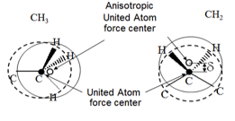
To take better stock of the influence of hydrogen atoms in United Atoms potentials, some experts have proposed shifting the force center to an intermediate position between the major atom and the related hydrogen atoms [16]. In this approach, referred to as “Anisotropic United Atoms” or AUA, the CH ₂force center is thus located on the external bisector of the C-C-C angle and the CH ₃force center is located on the C-C axis. The distance from the force center to the major atom is a parameter specific to the group under consideration. The separation distances in equations (1) and (2) are then counted between these force centers. The positions of the atomic nuclei are constructed exactly in the same way as with classical United Atoms models, with the same bending and torsion potentials, here shown for a CH ₃group (left) and a CH ₂group (right).

3.4.7. Embedded Atom Method Forcefields

Simulations for metallic systems often employ the ‘embedded atom model’ (EAM) description [17] where the energy of the system is represented by both two-body and density related terms.

\[U_{metallic} = \sum_{i=1}^{N-1} \sum_{j=i+1}^{N} V (r_{ij}) + \sum_{i=1}^{N} F (\rho_{i})\]

\[\rho_{i} = \sum_{j=1}^{N} \phi(r_{ij})\]

\(U_{metallic}\) is the total energy, \(i\) and \(j\) indicate each of the N atoms in the system, and \(r_{ij}\) is their interatomic separation. \(V(r_{ij})\) is a pairwise potential, \(F(\rho_{i})\) is the embedding function which depends on the electron density experienced by a given atom, and \(\phi (r_{ij})\) is an additional pairwise function, which represents the electron density at any atomic site based on its environment.

3.4.8. Stillinger-Weber and Tersoff Forcefields

The simulation of semiconducting materials has led to the development of forcefield forms, which can represent both bond angle deformation and the changing coordination of atoms. Here the simulated material possesses considerable covalent character, favoring the forcefield form typified by covalent descriptions, but additionally there is interest in surface restructuring and additional bonding subtleties, prompting interest in the development of forcefields able to handle variation in coordination numbers. Starting with Stillinger & Weber [18] and Tersoff [19], scientists have developed forcefield descriptions for semiconductors which combine elements of the EAM approach with the deformation from standard bond lengths employed in the covalent forcefields. The Stillinger-Weber forcefield form is summarized by Equations (11) - (13), where \(A, \epsilon, B, \sigma, p, q, a\) and \(\lambda\) are adjustable forcefield parameters, there being 8 such parameters for each distinct atom type covered by the forcefield.

(11)\[E = \sum_{ij} V_{2}(R_{ij}) + \sum_{jk} V_{3} \left( R_{ij}, R_{ik}, \theta_{ijk} \right)\]

(12)\[V_{2} = A \epsilon \left( B_{ij} \left( \dfrac{\sigma}{r_{ij}} \right)^{p} - \left( \dfrac{\sigma}{r_{ij}} \right)^{q} exp \left( \dfrac{\sigma}{r_{ij} - \alpha \sigma} \right) \right)\]

(13)\[V_{3} = \lambda (cos\theta - cos\theta_{0})^{2} exp \left( \dfrac{\lambda \sigma}{r_{ij}-a\sigma} \right) exp \left( \dfrac{\lambda \sigma}{r_{ik}-a\sigma} \right)\]

As can be seen from Equation (11) the essential form of the Stillinger-Weber forcefield is the summation of two-body interactions, across all pairs of atoms in the system, augmented with three-body terms, which encompass all triplets of atoms in the system. Both the two-body term (12) and the three-body term, Eq. (13) are damped by exponential functions according to the separation of the atoms involved in the interaction, which implicitly incorporates an effect the system density on the forcefield. This damping term also makes it possible to truncate interactions to zero at a separation distance governed by the \(a\) parameter for both two-body and three-body terms. Additionally, the Stillinger-Weber forcefield does not require a fixed connectivity for the constituent atoms in the system, as the sums of Eq. (11) extend to cover all possible pairs and triplets of atoms within the system.

3.4.9. Embedded Atom Methods, Stillinger-Weber, and Tersoff Forcefields in MedeA

To use EAM, Stillinger-Weber, or Tersoff forcefields, you first construct a structural model, read the appropriate forcefield file into MedeA, and then assign Forcefield atom types and Forcefield charges. In general with these forcefields, there will be one atom type per element in the simulation system. However, the procedure used to prepare a system for simulation is identical to that employed for organic systems.

[1]	William L Jorgensen, David S Maxwell, and Julian Tirado-Rives, “Development and Testing of the OPLS All-Atom Force Field on Conformational Energetics and Properties of Organic Liquids,” Journal of the American Chemical Society 118, no. 45 (January 1996): 11225-11236.

[2]	William L Jorgensen, J Chandrasekhar, and J D Madura, “Comparison of Simple Potential Functions for Simulating Liquid Water,” Journal of Chemical Physics 79 (1983): 926-935.

[3]

JL Rivail, Eléments De Chimie Quantique à L’usage Des Chimistes, Savoirs actuels. (EDP Sciences, 2000). William C Swope, Hans W Horn, and Julia E Rice, “Accounting for Polarization Cost When Using Fixed Charge Force Fields. I. Method for Computing Energy,” Journal of Physical Chemistry B 114, no. 26 (July 8, 2010): 8621-8630.

[4]	B M Axilrod and E Teller, “Interaction of the Van Der Waals Type Between Three Atoms,” Journal of Chemical Physics 11, no. 6 (1943): 299.

[5]	William L Jorgensen, David S Maxwell, and Julian Tirado-Rives, “Development and Testing of the OPLS All-Atom Force Field on Conformational Energetics and Properties of Organic Liquids,” Journal of the American Chemical Society 118, no. 45 (January 1996): 11225-11236.

[6]

MG Martin and IJ Siepmann, “Transferable Models for Phase Equilibria 1. United-Atom Description of N-Alkanes,” Journal of Physical Chemistry B 102 (1998): 2569; MG Martin and IJ Siepmann, “Novel Configurational-Bias Monte Carlo Method for Branched Molecules. Transferable Potentials for Phase Equilibria. 2. United-Atoms Description of Branched Alkanes,” Journal of Physical Chemistry B 103 (1999): 4508; Katie A Maerzke, Nathan E Schultz, Richard B Ross, and J Ilja Siepmann, “TraPPE-UA Force Field for Acrylates and Monte Carlo Simulations for Their Mixtures with Alkanes and Alcohols,” Journal of Physical Chemistry B 113, no. 18 (May 7, 2009): 6415-6425.

[7]	Nicolas Ferrando, Véronique Lachet, Jean-Marie Teuler, and Anne Boutin, “Transferable Force Field for Alcohols and Polyalcohols,” Journal of Physical Chemistry B 113, no. 17 (April 30, 2009): 5985-5995.

[8]	H Sun, “COMPASS: an Ab Initio Force-Field Optimized for Condensed-Phase -Overview with Details on Alkane and Benzene Compounds,” Journal of Physical Chemistry B 102, no. 38 (September 1998): 7338-7364.

[9]	Jeffrey R Errington and Athanassios Z Panagiotopoulos, “Phase Equilibria of the Modified Buckingham Exponential-6 Potential From Hamiltonian Scaling Grand Canonical Monte Carlo,” Journal of Chemical Physics 109, no. 3 (1998): 1093.

[10]	Angela Di Lella, N Desbiens, Anne Boutin, I Demachy, Philippe Ungerer, et al., “Molecular Simulation Studies of Water Physisorption in Zeolites,” Physical Chemistry Chemical Physics 8, no. 46 (2006): 11.

[11]	(1, 2) Chang Lyoul Kong, “Combining Rules for Intermolecular Potential Parameters. II. Rules for the Lennard-Jones (12-6) Potential and the Morse Potential,” Journal of Chemical Physics 59, no. 5 (1973): 2464.

[12]	(1, 2, 3) Marvin Waldman and A T Hagler, “New Combining Rules for Rare Gas Van Der Waals Parameters,” Journal of Computational Chemistry 14, no. 9 (September 1993): 1077-1084.

[13]	Soren Toxvaerd, “Equation of State for Alkanes II,” Journal of Chemical Physics 107 (1997): 5197.

[14]	William L Jorgensen, JD Madura and Carol J Swenson, “Optimized Intermolecular Potential Functions for Liquid Hydrocarbons,” Journal of the American Chemical Society 106 (1984): 6638.

[15]	Nicolas Ferrando, V\({\acute{e}}\)ronique Lachet, Jean-Marie Teuler, and Anne Boutin, “Transferable Force Field for Alcohols and Polyalcohols,” Journal of Physical Chemistry B 113, no. 17 (April 30, 2009): 5985-5995.

[16]	Soren Toxvaerd, “Molecular Dynamics Calculation of the Equation of State of Alkanes,” Journal of Chemical Physics 93, no. 6 (1990): 4290. Soren Toxvaerd, “Equation of State for Alkanes II,” Journal of Chemical Physics 107 (1997): 5197.

[17]	Murray Daw and M Baskes, “Embedded-Atom Method: Derivation and Application to Impurities, Surfaces, and Other Defects in Metals,” Physical Review B 29, no. 12 (June 1984): 6443-6453.

[18]	Frank H Stillinger and Thomas A Weber, “Computer Simulation of Local Order in Condensed Phases of Silicon,” Physical Review B 31, no. 8 (1985): 5262-5271.

[19]	J Tersoff, “New Empirical Approach for the Structure and Energy of Covalent Systems,” Physical Review B 37, no. 12 (1988): 6991-7000.

download:pdf