2.15. MedeA GIBBS

Contents

Overview
Basic Workflow
Launching and Analyzing Gibbs Computations
Results
Variables for Computed Properties

download:	`pdf`

2.15.1. Overview

MedeA GIBBS is aimed at computing the equilibrium properties of fluids by molecular simulation, using a Monte Carlo method in cubic, parallelepipedic or even non-orthorhombic simulation boxes. It has the following main features:

Determination of phase properties. Statistical ensembles: NVT, NPT, semi-grand canonical, osmotic
Adsorption through $\mu$VT simulation (Grand canonical ensemble), imposing an external field defined on a grid. Among other applications, it allows you to simulate the adsorption of molecules in microporous crystalline solids of cubic or orthorhombic structure.
Calculation of fluid phase equilibria, either two-phase (L-V, L-L) or multiphase (L-L-V…), using the Gibbs ensemble at imposed pressure or imposed global volume, without an explicit interface, but one separate simulation box per phase.

Unlike Molecular Dynamics, Monte Carlo methods do not aim at describing system evolution with time. Instead, Monte Carlo methods sample the possible configurations of the system in a way that satisfies the conditions of thermodynamic equilibrium on average, provided the structure of molecules and their interaction energy is known (see Section Monte Carlo methods ). Consequently, some post-processing features of the GIBBS menu (Continue a Run, Convergence, View configuration(s), View adsorption graphs, Cations location analysis) are specific to this tool while they are not fundamentally different from those of MedeA LAMMPS.

MedeA GIBBS works on pure fluids as well as multi-component mixtures. The possible types of molecules are:

rigid molecules
fully flexible molecules, either linear, branched or cyclic
semi-flexible molecules, with a rigid part and a flexible part

The following forms of energy may be accounted for:

dispersion-repulsion energy (Lennard-Jones or exp-6 centers of force)
electrostatic energy (partial electrostatic charges)
stretching, bending and torsion energy (flexible molecules only).

Note

Polarization energy, the action of the electrostatic field on the force centers, considered as polarizable, is not considered explicitly in most forcefields.

In a way, similar to many studies of adsorption or phase equilibria, MedeA GIBBS is most efficient with United Atom forcefields, such as TraPPE-UA or AUA. In such forcefields the hydrogens are generally lumped onto a heavy atom, for example a methyl group may be considered as one united-atom.

In the case of rigid molecules, any coordinates can be attributed to dispersion-repulsion centers and electrostatic charges. Any forcefield (United Atoms or All Atoms) can be used for such molecules. This means that electric charges can be placed outside atomic centers. In small molecules like H₂, N₂, O₂, H₂S, H₂O this allows an excellent representation of molecular interactions.

In order to simulate efficiently the various statistical ensembles and molecular types, more than 10 types of Monte Carlo moves are available. They use the pre-insertion and rotational bias for rigid molecules, and configurational bias for flexible molecules (see section Statistical Bias Monte Carlo moves).

MedeA GIBBS works in batch mode: data files are read in and result files are written out. A single job may comprise several tasks (for instance two tasks for building the grids, followed by two tasks for the simulation of adsorption at two fugacity levels). Each simulation is usually decomposed into several runs, which may include different Monte Carlo move probabilities, frequency of result storage, or the number of iterations, all under user control.

The main average properties are computed and printed in the Job.out file of the run.
For phase equilibria involving more than two components, the average composition of each phase is also determined and printed in Job.out.
In $\mu$VT simulations, the heats of adsorption are computed and printed in Job.out.
The GIBBS computations are generally followed by a specific post-processing step. The specific options are thus part of the GIBBS menu:
Gibbs >> Continue a run (for extending the run if convergence is slow)
Gibbs >> Convergence (for visualizing convergence of energy versus number of steps)
Gibbs >> View configuration (view molecules and/or solid in the stored configurations)
Gibbs >> View adsorption graphs (view adsorption isotherm)
Gibbs >> Cations location analysis

2.15.2. Basic Workflow

The purpose of the present section is to introduce the first-time user to the various steps involved in simulations with the MedeA GIBBS software, which may be useful as several types of input files are required and several output files are generated in any simulation.

Note

The legacy file containing the forcefield parameters used by GIBBS is updated with each revision of MedeA. You cannot change the name of this file, but you can still edit it, provided you store if in a different folder, e.g Forcefields/custom/. It is important that the potparam.dat file is the same on the machine with the GUI and the JobServer, otherwise MedeA GIBBS will fail or provide generate results based on the parameters present on file on the JobServer.

Note that the units in potparam.dat are as follows:

Distances (ex. Lennard-Jones diameter, AUA offset) in ${\mathring{\mathrm{A}}}$
Energy parameters (Lennard-Jones epsilon) are expressed as $U/k_{B}$, i.e. they scale like temperature, and their unit is K.
Molecular mass in g/mol

Note

Molecular mass does not influence the course of the Monte Carlo simulation, as it does not influence the potential energy terms. However it plays an important role in property calculations.

In the case of united atoms (Trappe-UA, AUA) the molecular mass attached to the force center includes the mass of constituting atoms (e.g. 12.01 g/mol for C, 13.01 g/mol for CH, 14.02 g/mol for CH₂). Hydrogens are not considered explicitly in the course of the simulation, but their positions can be reconstructed from the position of carbons if required.

2.15.2.1. Defining Molecular Species

Molecules present in a Monte-Carlo run are defined by molecule.sci files. One file per species should be available. A molecule.sci file may be created by File >> New non periodic structure. Through File >> Open, the user may also open an already created molecule file.

Several molecular files used with GIBBS are stored in MD/Structures/Gibbs and its subfolders.

Although forcefield assignment is available, it is advised that users use first the molecular files of this folder, if present. This is particularly advised in the case of potential models for small molecules, which contain frequently off-atom Lennard-Jones sites or electrostatic charges. Charges are expressed in multiples of electron charge and distances are in ${\mathring{\mathrm{A}}}$.

For instance, the TIP4P model of water (file H2O - TIP4P.sci) involves one Lennard-Jones site on the oxygen, but no such site on hydrogens. Two positive electrostatic charges are set on the hydrogens, and a negative charge is located at 0.15 ${\mathring{\mathrm{A}}}$ of the oxygen nucleus.

Another example is the molecule of methane (CH₄). In the united atom description, a single Lennard-Jones site is used ($\sigma$ = 3.7327 ${\mathring{\mathrm{A}}}$, $\epsilon$ = 149.92 K), without electrostatic charges. The molecular mass (16.043 g/mol) refers to one carbon + four hydrogens. Hydrogens are not considered (they appear as blank fields in the “Forcefield Atom type” of the spreadsheet of the molecular builder.)

Several formats can be read in (i.e. *.car, *.xyz, *.xmol)., but the association with a specific force field is only saved in the sci format. The global electrostatic charge of a molecule should be neutral, $0 \pm 10^{-5} e$.

2.15.2.2. MedeA GIBBS Flowcharts

By clicking on Gibbs >> Define computation, a new window pops, where the user can design in just a few steps a complete flowchart where all the simulation parameters and details are set.

In the Materials Design Flowchart (gray color boxes for stages):

Start must be selected as the first stage.
Set Variables brings up an optional stage: Here you can define as many control variables as for all following simulation stages (i.e. temperature, pressure, …).
Gibbs: Monte Carlo brings up the main simulation stage. A new window pops when the user opens this stage. In this stage, the user can design the main Gibbs flowchart.

The MedeA GIBBS flowchart (green color boxes) should contain the following stages:

2.15.2.2.1. Start Stage

The first part of any flowchart is the Start stage.

Stages show the bare minimum of options, all other parameters are set to their default values and their values are accessible through “Advanced Settings” in each stage.

2.15.2.2.2. Initialization

Initialization is achieved through the Initialize Gibbs stage. This sets parameters for the interatomic potential: the method for dealing with electrostatic charges, the cutoff and minimum non-bond distance. These parameters control the way that the interactions between the system particles are computed. Default values are proposed by MedeA GIBBS, but tests should be made depending on the specific systems to be studied. Note that zero or negative values for the cut-off are understood as selecting half the box length as cut-off (in case of non-cubic boxes, the smallest box length is selected).
Random seed: -1 means that a new seed for the random generator is defined for clock time (used if the simulation must be repeated with different parameters). 0 means that the standard seed is taken (two successive runs with the same input on the same machine will provide the same results)

Note

Include intramolecular electrostatic has no impact on rigid molecules, but can be required for long, flexible molecules with more than one functional group. Of course this increases the computation time.

After initialization of GIBBS, you chose the type of simulation: Single Phase Properties, Phase Equilibria & Properties or Adsorption.
- Single phase properties refers to monophasic fluid simulations
  
  in the NPT, NVT, or Semigrand Canonical ensembles of either pure compounds or mixtures. It allows also the determination of gas solubility constants in the fluid through Widom test insertions.
- Phase equilibria & Properties refer to the simulations of phase equilibrium without explicit interface in the Gibbs ensemble. MedeA GIBBS will then create one simulation box per phase.
- Adsorption refers to simulations in the Grand Canonical ensemble ($mu$VT) where fluid molecules interact with a microporous solid

Depending on the type of simulation chosen, the parameters that refer to the corresponding ensemble must be set (temperature, pressure, chemical potential etc.). Also, in this stage, the flowchart defines the molecule.sci files (one for each species of the system). There are two possible ways to read in the molecule.sci files; if open in MedeA, click on Add component from MedeA, if the file is saved on the computer, use Add component from a file.

Initial configuration: in contrast to LAMMPS or VASP, GIBBS does not require the initial positions of all molecules in the NVT or NPT ensembles. MedeA GIBBS fills the simulation box with the number of molecules that the user has specified (they are placed on a regular lattice with random orientations).

Note

Avoid problematic overlap of molecules in dense phases (such as a liquid phase in the NPT ensemble) by starting at a low density (typically 20 to 60% of the expected final density) and check that the intermolecular attraction is sufficient to allow the simulation box to shrink.

The final part of the simulation is one or more Run stages. Here the number of total steps for the simulation run, the intervals for writing (in the corresponding output files) the configuration, the main averages, the restart file, etc are defined. Also, the various move probabilities are defined here. Depending on the ensemble in which the simulation takes place, different types of Monte Carlo moves are available:
- Internal moves:
  1. regrowth of a molecule (flexible and semi-flexible molecules, all ensembles), based on configurational bias
  2. internal rotation of one atom in a chain (around the axis of its immediate neighbors)
  3. pivot (rotation of a part of the molecule around an axis crossing a center, branched and semi-flexible molecules, all ensembles)
  4. reptation (linear flexible and semi-flexible molecules, all ensembles), including configurational bias
  5. concerted rotation (linear flexible and semi-flexible molecules, all ensembles)
  6. double bridging (linear flexible and semi-flexible molecules, all ensembles)
  7. internal double rebridging (linear flexible and semi-flexible molecules, all ensembles)
  8. stretching move (atomic translation)
- Rigid moves:
  1. rigid body translation of a molecule (all molecular types, all ensembles),
  2. rigid translation and rotation (displacement move, displacement of a molecule by moving it to a random position and orientation in the same box)
  3. rigid body rotation of a molecule (all molecular types, all ensembles)
  4. exchange of two molecules,
  5. swap of two molecules of different types
- Transfer moves:
  1. molecular transfers between phases (Gibbs ensemble)
  2. insertions and destructions (Grand Canonical ensemble), including Widom test insertions
- Volume changes
  
  Depending on the type of molecules (i.e. flexible or rigid) certain types of moves may bring up error messages when set to non-zero values. Some examples are provided in the FAQ section.

Note

It is important that averages are calculated for a system has been well equilibrated, i.e. when long term averages of energy fluctuations (as well as other property fluctuations) do not show significant drift.

Note

You do not need to set any of the move probabilities by hand. MedeA assigns automatically default values and weights on the types of moves that are relevant to the molecules present in your simulation and their specific structure, as well as the type of simulation (the statistical ensemble).

Subsequent Run stages may be used to have an equilibration run, followed by a production run. Each Run stage, after the first one, will use as an initial configuration the last configuration of the previous Run stage.

2.15.2.2.3. Simulation of a Monophasic Fluid in the NVT or NPT Ensemble

Single Phase Properties offers NVT or NPT ensemble: In these ensembles, only input files listed at the beginning of this section are required. The rest of the input files that are necessary, to start the simulation, are created automatically, when the user fills in the corresponding fields in the simulation flowchart.

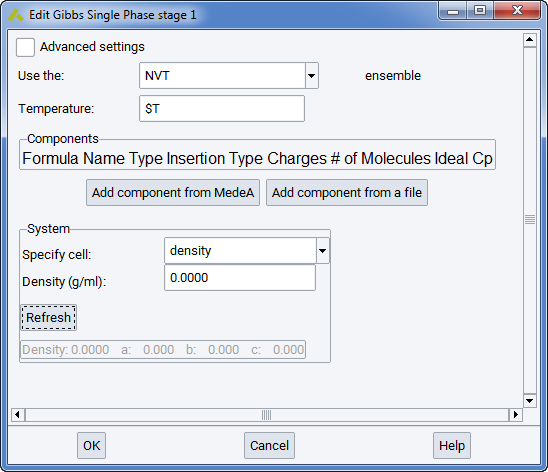
Note that $T refers here to the variable T entered for Temperature in the Set Variables stage of the flowchart. Similarly, $P refers to the variable P for Pressure.

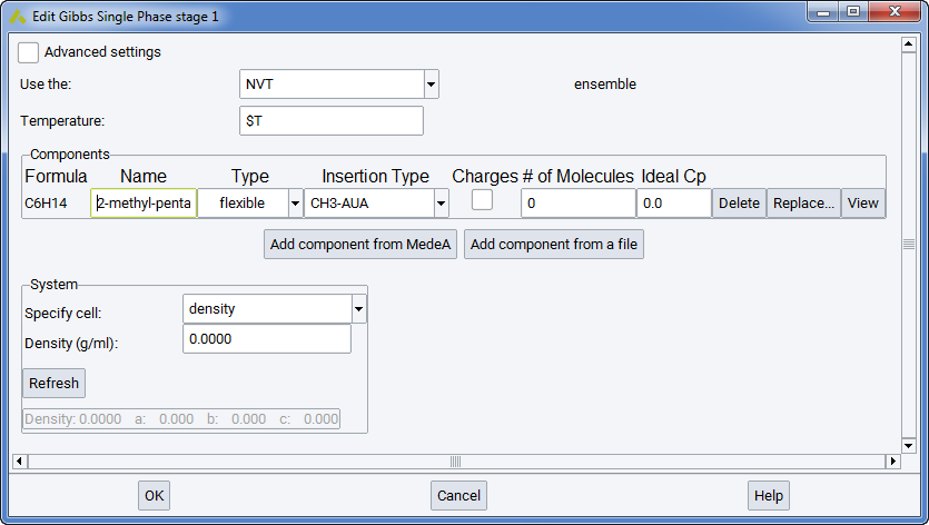
In the Components section you can define different components and their occurrences. When a new component is added from MedeA or from a file, it appears as a new line in the frame. The column Name refers to the identification of this component by MedeA. The column Type refers to the molecular structure (flexible, rigid, or semi-flexible). This should not be changed from the molecule.sci file, as it refers to different ways of defining molecular structure in MedeA GIBBS (see section Defining molecular species)

When calculating a solubility constant for a given molecule, the molecular type of the solute should be entered in the list, and test insertions should be explicitly added with a reasonable frequency in the MC moves section of the Run stage.

The Insertion type refers to the force center that is used to test positions of the solute in the pre-insertion bias. The diameter of this force center should not be larger than the smallest dimension of the molecule. The Insertion type field is filled by a default value in MedeA.

The column charges informs the user of partial electrostatic charges in the molecules he has selected. Expert users may decide to neglect electrostatic charges for either molecule, but this is not advised in the general case.

The column ideal cp refers to the ideal heat capacity of the pure component considered, at the temperature considered, in J/mol/K. This input is needed when thermodynamic properties are computed from fluctuations (see section Thermodynamic derivative properties for more details). However, it does not influence the course of the simulation, as it is used at the post-processing stage only.

In the Components section you can define the system size and shape in a number of different ways. More specifically:

Specify cell provides a variety of options for controlling the size of the initial configuration of the system. Thus, for example, choosing Specify cell density will produce cubic cells in which the cell edges are determined based on the overall composition and density. Similarly, choosing Specify cell density,c will create tetragonal cells based on the density and specified c dimension, while choosing Specify cell a,b,c creates orthorhombic cells using the a, b and c lengths provided (in which case the density cannot be specified independently since it is fixed by the composition).

The full set of options for Specify cell… is as follows:

Density: Density is provided in units of g/mL and can be either a numeric value or a previously defined variable (e.g. $d).
density,a Density is provided in units of g/mL and can be either a numeric value or a previously defined variable (e.g. $d). The side of the simulation box (a) is provided in units of ${\mathring{\mathrm{A}}}$ and can only be numeric values.
density,b Density is provided in units of g/mL and can be either a numeric value or a previously defined variable (e.g. $d). The side of the simulation box (b) is provided in units of ${\mathring{\mathrm{A}}}$ and can only be numeric values.
density,c Density is provided in units of g/mL and can be either a numeric value or a previously defined variable (e.g. $d). The side of the simulation box (c) is provided in units of ${\mathring{\mathrm{A}}}$ and can only be numeric values.
density,a,b Density is provided in units of g/mL and can be either a numeric value or a previously defined variable (e.g. $d). The sides of the simulation box (a and b) are provided in units of ${\mathring{\mathrm{A}}}$ and can only be numeric values.
density,a,c Density is provided in units of g/mL and can be either a numeric value or a previously defined variable (e.g. $d). The sides of the simulation box (a and c) are provided in units of ${\mathring{\mathrm{A}}}$ and can only be numeric values.
density,b,c Density is provided in units of g/mL and can be either a numeric value or a previously defined variable (e.g. $d). The sides of the simulation box (b and c) are provided in units of ${\mathring{\mathrm{A}}}$ and can only be numeric values.
a,b,c The sides of the simulation box (a, b, c) are provided in units of ${\mathring{\mathrm{A}}}$ and can only be numeric values.
volume: The volume of the simulation box is provided in units of ${\mathring{\mathrm{A}}}$^3 and can only be a numeric value.
a,b,c,alpha,beta,gamma The angles of the simulation box (${\alpha}$, ${\beta}$, ${\gamma}$) are provided in units of degrees and can only be numeric values.

Once the flowchart is ready, the user may run the simulation. At first, a series of consistency checks on the input data is performed and related messages are written in the gibbs.log output file. If the consistency tests are successful, the code proceeds by writing several types of result files.

First types of result files are history files, the main of which are Aavg1.res Aavg2.res…. These files contain instantaneous values of energy, volume or pressure taken at specific times during the Monte Carlo simulation. Ajt1.res contains the observed fluctuations and allows computing thermodynamic derivative properties like thermal expansivity based on these fluctuations.

The code is also writing two types of files: the configuration file (conf1.res) and the restart files (restart-odd.res and restart-odd.res) which provides a snapshot of the last system configuration. Other files, characterized with extension .mol (as Aconf1.mol) allow visualizing a snapshot of the molecules in the last configuration. MedeA’s post-processing utility reads the content of Aavg1.res files to compute average volume, density or pressure, together with the estimated statistical uncertainties.

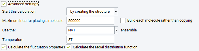
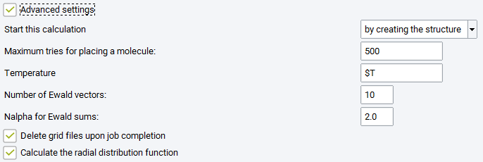
Advanced Settings

Maximum tries: maximum number of orientations tested for building the initial box with the requested number of molecules (this is corresponding to parameter indexmax_initconf, in the control.dat GIBBS input file).

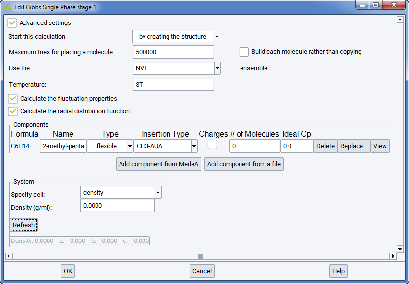
Build each molecule rather than copying: checking this box means that the random number generator will generate new molecular conformations for each molecule when building the initial box with the requested number of molecules.

Two optional boxes may be checked to generate more analysis: Calculate the fluctuation properties (i.e. thermodynamic derivative properties, see section Thermodynamic derivative properties) and Calculate the radial distribution function, a standard way to characterize the structure of liquids.

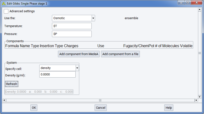
2.15.2.2.4. Simulation of a Monophasic Fluid in the Osmotic Ensemble

The osmotic ensemble is a way to simulate phase equilibria with polymeric materials without simulating the liquid phase. There may be any number of molecular types for the fluid and the polymer. It is aimed at computing the solubility of fluid components in the polymers under a specific stress condition and fluid pressures. It should be noted that stress may be different from fluid pressure. The osmotic ensemble may also be used to compute fluid phase equilibria involving a heavy component that cannot enter the light phase, for instance an equilibrium between a gas and a heavy alkane under pressure. In this case, the stress variable in the osmotic ensemble simulation must be identical to the pressure in the preliminary NPT simulation of the light phase.

Single Phase Properties offers access to the Osmotic ensemble. In this ensemble, only input files listed in the beginning of this section are required. The rest of the input files that are necessary, in order to start the simulation, are created automatically, when the user fills in the corresponding fields in the simulation flowchart. Alternatively, the simulation can begin from the resulting configuration of a past simulation (e.g. from a resulting configuration of a previous NPT compression of a heavy compound, with zero or very small inclusion of a light compound).

Note

$T refers here to the variable T, entered for Temperature in the Set Variables stage of the flowchart. Similarly, $P refers to the variable P for the total stress entered again in Set Variables stage of the flowchart.

In the Components section, you can define different components and their occurrences. When a new component is added from MedeA or from a file, it appears as a new line in the frame.

The column Name refers to the identification of this component by MedeA. The column Type refers to the molecular structure (flexible, rigid, or semi-flexible).
The column Insertion type refers to the force center that is used to test positions of the solute in the pre-insertion bias. The diameter of this force center should not be larger than the smallest dimension of the molecule. The Insertion type is chosen by MedeA.
The column Charges informs the user of partial electrostatic charges in the molecules he has selected. Expert users might decide to neglect electrostatic charges for a molecule, but this is not advised in the general case.
The column Fugacity/ChemPot refers to the imposed fugacity or chemical potential (respectively) of each component, as in the Grand Canonical and semi-grand canonical ensemble simulations. Before a simulation is made in this ensemble, the user should determine the chemical potentials of the fugacities in the fluid phase by an NPT simulation involving Widom test insertions. As the fugacity (or the chemical potential) play the same role in this ensemble as in GCMC simulations, it is mandatory to use insertion and deletion moves in the Run stage(s).
The column Volatility refers to the identification of the volatile component(s) in the system, i.e. the compounds of which the total number in the system may vary (these should always have a total charge equal to zero), and the non-volatile (i.e. the heavy compounds of which the total number in the system will remain constant throughout the simulation). Consequently, the Volatility column will control the way the insertion/deletion move weights are selected, for on the components of the system.

Once the flowchart is ready, the user may run the simulation. At first, a series of consistency checks on the input data is performed and related messages are written in the gibbs.log output file. If the consistency tests are successful, the code proceeds by writing several types of result files.

First types of result files are history files, the main of which are Aavg1.res Aavg2.res …. These files contain instantaneous values of energy, volume or pressure taken at specific times during the Monte Carlo simulation.

The code is also writing two types of output files: the configuration file (conf1.res) and the restart files (restart-odd.res and restart-odd.res) which provide a snapshot of the last system configuration. Other files, characterized with extension .mol (as Aconf1.mol) allows visualizing a snapshot of the molecules in the last configuration. MedeA’s post-processing utility reads the content of Aavg1.res files to compute average volume, density or pressure, together with the estimated statistical uncertainties.

Advanced settings

Maximum tries: maximum number of orientations tested for building the initial box with the requested number of molecules.

Build each molecule rather than copying: checking this box means that the random number generator will generate new molecular conformations for each molecule when building the initial box with the requested number of molecules.

Two optional boxes may be checked to generate more analysis: Calculate the fluctuation properties (i.e. thermodynamic derivative properties, see section Thermodynamic derivative properties) and Calculate the radial distribution function, a standard way to characterize the structure of liquids.

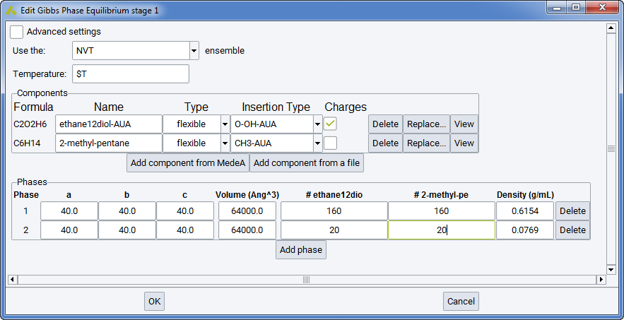
2.15.2.2.5. Simulation of Fluid Phase Equilibria in the Gibbs Ensemble

A Gibbs ensemble simulation requires basically the same input files (molecular structure files) as the monophasic NVT or NPT simulations considered above. The specification of the number of phases in the Gibbs >> Phase Equilibria & Properties flowchart stage is sufficient to ask for e.g. a two-phase simulation.

This means that two simulation boxes with different densities will be considered for two-phase equilibria, three simulation boxes for three-phases. Each box must be representative of the phase considered, i.e. it should be homogeneous (as the interface is not explicitly modeled) and should contain at least 2-3 molecules of each type.

Among the practical differences between phase equilibrium and monophasic simulations, the following are most important:

provide the initial number of molecules in each box (columns “# molecule1”, “#molecule2”, etc.)
provide the initial size (columns a, b and c, in ${\mathring{\mathrm{A}}}$) for each simulation box (or alternatively, the initial density in g/cm ³)
allocate a significant frequency to Monte Carlo transfer moves AND to volume change moves in the definition of the Run stages
You cannot apply the Gibbs ensemble NPT to the phase equilibrium of a single component, as this would not respect the phase rule. This is possible only in the NVT ensemble, when the sum of phase volumes is imposed.

These selections can be quite sensitive and critical for the successful convergence of your phase equilibrium calculations. For instance, the phase densities and compositions of a binary systems will tend toward the same values in both boxes if the average composition of the systems falls in the monophasic domain in the P, x diagram. In order to converge toward different properties in the vapor and liquid boxes, the composition should be well inside the liquid-vapor coexistence domain.

A Gibbs ensemble simulation at imposed volume or imposed pressure is made automatically when there is more than one phase. As specific differences between phase equilibrium and monophasic simulations, you must allocate a significant frequency to transfer Monte Carlo moves, and provide the initial number of molecules and box size for each simulation box. These selections can be quite sensitive and critical for successful calculations.

The output files are qualitatively the same as in monophasic fluid simulations, except that all those pertaining to a single simulation box are duplicated. Thus result files are Aavg1.res, Aconf1.mol, … for the first fluid phase and Bavg1.res, Bconf1.mol, … for the second fluid phase. As the chemical potential is a byproduct of Gibbs ensemble simulations, the chemical potentials in both boxes are gathered in the Cp1.res file.

Pressure equilibrium is reached if there is a significant overlap of the error bars of the virial pressure in phase 1 and the virial pressure in phase 2. Chemical equilibrium is reached when a significant number of Monte Carlo transfer moves have been accepted for each molecular type. These statistics are available in the final1.res file for run 1, final2.res for run 2, etc.

In simulations of phase equilibrium at imposed volume, post-processing provides the coexisting densities and the virial pressure in each phase (see section Thermodynamic integration for fluid phase equilibria). Usually the uncertainty of the virial pressure is significantly larger in the liquid phase (several bars). Then the vapor phase pressure is a more reliable estimation of the equilibrium pressure.

In simulations at imposed pressure P, it should be checked that the virial pressure of each phase is in agreement with P (i.e., that the error bar on virial pressure contains P).

In simulations of a binary mixture at imposed pressure, the equilibrium mole fractions and densities are also printed in the Job.out file.

Advanced Settings

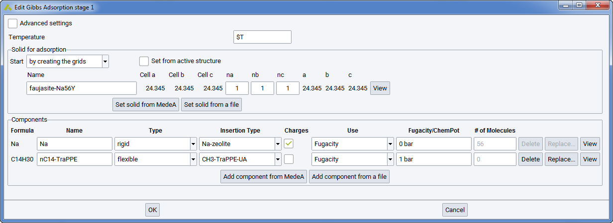
2.15.2.2.6. Simulation of Adsorption in the Grand Canonical Ensemble

Compared with the above-mentioned simulations of fluid phases, the simulation of adsorption in microporous solids differs due to the use of the Grand Canonical ensemble and the treatment of the solid as an external forcefield. However, the way of defining the components of the system are identical to bulk fluid phases.

A Grand Canonical simulation is characterized by setting Gibbs >> Adsorption in the flowchart and by specifying the chemical potential of each molecular species, since this is an imposed parameter in this ensemble. Alternatively, the user may enter fugacity, which is equivalent to partial pressure at low pressure, instead of chemical potential (see sections Forcefields for materials simulations and Evaluation of the Chemical Potential by Test Insertions). In MedeA GIBBS, the unit for chemical potential is Kelvin (as it is expressed in $\mu /k_{B}$). Fugacities may be entered as mPa, Pa, kPa, bar, atm.

The treatment of the solid is by far the most characteristic feature of the simulation of adsorption. Indeed, it is a common procedure to consider the solid as rigid, and this allows reducing considerably computer time through a preliminary computation of the interaction energy between the guest molecules and the microporous solid.

For this purpose, you must provide a unit cell of the solid (section Solid for Adsorption in the Gibbs Adsorption stage) such as it can be obtained from crystal databases of InfoMaticA. Note that MedeA GIBBS will consider the unit cell as P1 symmetry and requires an assigned forcefield type and charge for each atom of the unit cell, according to the forcefield used.

The preliminary computation of interaction energies is made by MedeA GIBBS in a specific task before starting the Monte Carlo iterations. It makes use of the solid coordinates file together with a specific parameter set as input and generates different energy grid files. These grid files are named this way because they contain the potential energy on the nodes of a grid with regular spacing in x, y, z covering the unit crystal cell. The default grid spacing is 0.2 ${\mathring{\mathrm{A}}}$. For a typical box size of 25x25x25 ${\mathring{\mathrm{A}}}$, it implies the calculation and storage of 125³ energy values, i.e. more than 2.5 million points. Such files are commonly more than 100 Mb, and they may cause memory problems if spacings lower than 0.2 ${\mathring{\mathrm{A}}}$ are considered. Therefore, you can select Delete grid file, which deletes the grid files after usage in the current job.

The solid unit cell should be selected as small as possible, because the simulation box can contain multiple unit cells. Various grid files can be generated depending on the type of potential energy to be considered:

the dispersion-repulsion energy grid file (generally one such file per force center of the adsorbed molecules),
the electrostatic energy grid file (a unique file corresponding to the interaction of a unit point charge with the solid).

Using a simulation box larger than the unit cell is possible through the parameters na, nb and nc of the panel (integer values). The resulting length of the simulation box along a, b and c directions is provided. You create a small model and assign forcefield parameters (or calculate the grid with VASP), and then use a larger cell, containing na x nb x nc cells.

The functional form of the zeolite-guest energy potential may be either Lennard-Jones or Buckingham (i.e. exponential repulsion and 1/r⁶ dispersion). Once the grid files are generated, they may serve to simulate the adsorption in the system considered by running MedeA-Gibbs simulation at various conditions of temperature and chemical potential, for pure components and mixtures as well. Making the grid files takes place as a separate task for each grid, preceding the actual Monte Carlo simulation. It takes place automatically, after all the necessary parameters have been defined and the input solid file has been provided in the GIBBS flowchart.

VASPtoGIBBS: generation of the electrostatic grid by VASP

The format of the electrostatic grid makes it possible to use a locpot file generated by a VASP single point analysis. Although it is not strictly required that VASP is used to optimize the solid structure, it is recommended (the electrostatic field would be erroneous if the atom nuclei do not occupy stable positions). It is of course recommended that a small unit cell be selected to minimize VASP computing time, and to use multiple unit cells to have a representative number of adsorbed molecules if needed.

Note

Be careful that the dispersion-repulsion grid is still needed when the locpot file from VASP is used.

Grand Canonical ensemble simulations involve specific moves, namely insertions and destructions of molecules, which should be attempted often enough (their frequencies are allocated by MedeA GIBBS and are typically 0.30). You can select other frequencies than proposed by MedeA, but enforce with Normalize that the sum of Move probabilities is equal to 1. The weight of the different molecules in each Monte Carlo move may be changed if the acceptance rate is low for a specific molecular type.

The output files generated by MedeA GIBBS are similar to bulk fluid simulations: Aavg1.res files provide the history of the number of molecules and energy with the progress of the Monte Carlo simulation, Aconf1.mol allows a graphic display of adsorbed molecule with rasmol, etc. Post-processing is also presenting a lot of common features with bulk fluid simulations in the NPT or NVT ensembles. The averages are provided in the file Job.out, particularly the average number of molecules as well as the evaluation of the isosteric heat of adsorption.

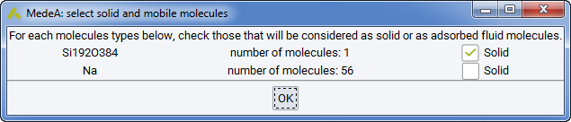
In some cases it may be useful to perform a Grand Canonical simulation of adsorption in a system that contains a rigid framework and guest molecules (for instance a faujasite zeolite and water molecules). Then, MedeA lists the identified solids or molecules, and asks you to select the adsorbates in the component stage below:

Advanced Settings

2.15.2.3. Adsorption Isotherms

The Adsorption isotherm stage consists in automating the simulation of several state points in the Grand Canonical ensemble at different values of chemical potential or fugacity. Its purpose is two-fold:

avoid that the user spends unnecessary time in launching several different Adsorption jobs to compare with experimental sorption isotherms,
organize the computations in such a way that the final stage of a simulation may be used to initialize the next point, allowing thus to simulate adsorption (increasing fugacities) and desorption (decreasing fugacities).

Creating the Adsorption isotherm stage is justified by their frequent occurrence in expressing adsorption data on microporous solids, either for characterizing their pore structure (BET analysis is based on nitrogen sorption isotherm at 77K) or their performance in adsorbing specific compounds.

It is also important to identify possible hysteresis effects (i.e. different paths on adsorption and on desorption) and optimizing sampling efficiency.

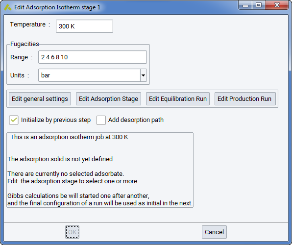
The first panel, Isotherm parameters, allows you to see the important parameters at one glance: Temperature, the fugacity values, the Adsorption solid. It contains also four boxes featuring.

Edit general settings: opens the window Edit Gibbs Initialize Stage (Ewald parameters, cut-off, functional forms of Nonbond Forcefield terms)
Edit adsorption stage: opens the window Edit Adsorption Stage (selection of the solid, number of unit cells, grid spacing, components). Note that adsorbed components are often called Adsorbates, while the solid is termed Adsorbent. Note that the practice to define molecules with better names than “Untitled” is useful in the long range…
Edit Equilibration run: opens the window Edit Gibbs Run Stage (display/selection of the number of Monte Carlo steps, Monte Carlo move frequencies, … of the equilibration run)
Edit Production run: opens the window Edit Gibbs Run Stage (display/selection of the number of Monte Carlo steps, Monte Carlo moves, … of the production run)

After defining the solid and all adsorbates, you will see a summary of Adsorption Isotherm conditions:

This is an adsorption isotherm job at 298K.
The grid will be created from the solid \* (C)88 (P1) ~CNT-(11,0)-semiconductor
Current adsorbate is: methane-Moeller
Gibbs calculations will be started independently,
And can run in parallel according to TaskServer availability.

2.15.3. Launching and Analyzing Gibbs Computations

Define computation:

This opens a flowchart and allows you to define the type of computation together with specific settings for each sampling run. Add a title to your computational job and submit with Run to the JobServer. Depending on your configuration, MedeA GIBBS runs efficiently on multiple processors with shared memory, thus speeding up your simulations. Depending on system size and architecture, this is very efficient with 4 to 16 cores.

Continue a run: Allows extending a computation based on the final configuration. A new run stage is added to the flowchart.

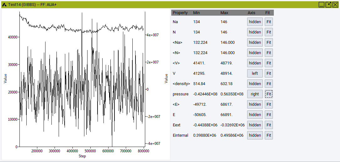
Convergence: Analyze properties and their averages over time:

Number of molecules A Na, overall number of molecules, N , Volume V, density, pressure, and energies.

View configuration(s):

While analyzing configurations from adsorption computations, you will be asked, “Merge configuration with adsorption solid?” to display the solid in addition to the adsorbate. You can use the combined system as the input structure for diffusion studies in LAMMPS.

View adsorption graphs: After an adsorption isotherm job has been completed (Gibbs: Adsorption Isotherm), you are able to view the sorption graphs and the isosteric heat of sorption as a function of fugacity.

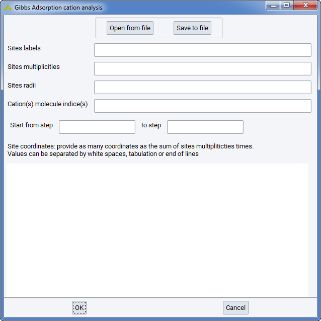
Cations location analysis: Cation location analysis can be performed in systems where cations have been allowed to move throughout the simulation, i.e. they were not considered part of the solid but part of the fluid, with zero insertion/deletion moves but non-zero translation moves. You will be prompted with a small wizard where you will need to specify the positions (sites) that you want to search for the existence of cations throughout the simulation or during a certain part of it. A confs*.res needs to be present in the simulation, to be analyzed. This file will exist if you have specified that average configurations are kept during the simulation run.

2.15.4. Results

The result filenames are written in the respective task directory and consist of a name and an extension:

.mol: visualization files
.res: files containing, at successive timesteps, the value of several physical quantities

In general, the filenames are like <Phase><Name><run>.<extension>, with exceptions explained below.

<Phase> is an uppercase letter corresponding to the simulation box: A for the first phase, B for the second and so on.

<Name> describes the file contents: avg corresponds to the average values of various physical quantities at successive timesteps.

<run> is the number of the run during which the file was generated.

Bavg3.res contains the average quantities for the third run and the second phase of the system.

2.15.4.1. Used Forcefield Parameters File (potparam.res)

The potparam.res file contains all the forcefield parameters, which are used in the current simulation. This file is written by default in each task directory.

2.15.4.2. Main Average Files

The names of these files are: Aavg1.res, Bavg1.res, Aavg2.res, Bavg2.res etc. The number at the end of the filename refers to the run number and the letter at the beginning of the filename refers to the corresponding phase.

These files contain the instantaneous values and the averages (computed by intervals) of various physical quantities. The length of these intervals (number of steps in between two averages recordings) is defined each Run stage of the flowchart, in the Intervals tab, in the Writing the main averages box.

The energies are given as $\epsilon$/k_B (as are the energy dispersion-repulsion parameters of the potparam.dat forcefield file) and therefore in temperature units, K.

Note

This file contains only potential energies; as kinetic energy is not part of a Monte Carlo simulation.

Average quantities recorded in this file are taken from the last interval, current quantities are taken from the last step. There are 19 columns in this file:

step number,
current number of type 1 molecules for this phase,
current number of molecules for this phase,
average number of type 1 molecules for this phase,
average number of molecules for this phase,
average total energy, including the long distance correction (K),
average electrostatic energy, including the grid-molecule electrostatic energy (K),
average grid-molecule energy: dispersion-repulsion and electrostatic (K),
average electrostatic grid-molecule energy (K),
current total energy, without the long distance correction (K),
current total intramolecular energy, without the long distance correction (K),
current induction energy (K), (not implemented)
current intramolecular energy (K),
average volume of the phase (${\mathring{\mathrm{A}}}$³)
current volume of the phase (${\mathring{\mathrm{A}}}$³)
average density of the phase (kg/m ³)
current pressure (Pa) (requires Calculate the pressure with the virial formula)
current dipole moment (requires induction computation - not implemented)
current energy due to the external field (in K) (requires external electric field - not implemented)
These files are used to visualize the evolution of these quantities. They are also used to compute the averages on a whole simulation, according to the convergence criteria, and printed at the Job.out file present in the job directory.

2.15.4.3. Composition Files (Acom1.res)

These files, with names such as Acom1.res, contain the molar fractions of each constituent. They are useful only for a system with three or more constituents. For a system with up to two constituents, the Aavg1.res file suffices for the determination of the phase composition.

2.15.4.4. Configuration Files (conf1.res)

There is one such file for each run (with names such as conf1.res, conf2.res….). They contain the information needed to restart a simulation from the last configuration of a previous run.

2.15.4.5. Run summary files (final1.res)

There is one such file for each run (with names such as final1.res, final2.res, etc.). For each type of possible moves, they contain the total number of attempts and successes.

Note

A summary of the attempted and performed moves, in each run and in each phase, is also provided in Job.out in the task directory.

2.15.4.6. Chemical potential files (Cp1.res)

These files contain averages collected at regular intervals for each run (with names such as Cp1.res, Cp2.res, etc.), if phase equilibrium is simulated. Each line contains the current step number and the chemical potential for each constituent in each phase.

These properties are not obtained by simple ensemble averages. The long term average is determined with specific statistical rules in MedeA GIBBS and reported in Job.out.

2.15.4.7. Visualization files (Aconf1.mol)

These files, with names such as Aconf1.mol, are written by default for each run (the number at the end of the filename refers to the number of the run).

2.15.4.8. Fluctuation files (Ajt1.res, Ajt2.res)

These files contain averages collected at regular intervals for each run if the Calculate the fluctuation properties checkbox is checked in the Gibbs stage (in a Single Phase Properties, or a Phase Equilibria & Properties, or an Adsorption simulation run). They are used to compute derived properties such as the Joule-Thomson coefficient.

Note

Derivation of the Joule-Thomson coefficient, isentropic compressibility, and total heat capacity, requires that the ideal $C_{p,id}$, which cannot be computed by Monte Carlo simulations and therefore should be provided for each component of the system in the Gibbs Stage.

These properties are not obtained by simple ensemble averages. The long term average is determined with specific statistical rules in MedeA GIBBS and reported in Job.out.

2.15.4.9. Radial Distribution Files (Agder1.res, Agder_elec1.res)

These files, with names such as Agder1.res, Agder_elec1.res, contain the radial distribution function g, calculated during the simulation run between all centers of forces in the Agder1.res file, or between all electrostatic centers in the Agder_elec1.res file. The partial g(r) are calculated at the same intervals as the intervals in which the main averages are recorded. These files are written only if the Calculate the radial distribution function checkbox is checked in the Gibbs stage (in a Single Phase Properties, or a Phase Equilibria & Properties, or an Adsorption simulation run).

2.15.4.10. Restart file (restart.dat)

The restart file contains, in binary form, the full simulation state at a given moment.

2.15.4.11. Isosteric Heat of Adsorption (in Job.out)

The Isosteric Heat of Adsorption and the Grid Isosteric Heat of Adsorption (Isosteric heat of adsorption at low coverage) are printed in the results part of Job.out, after the simulation has finished.

2.15.4.12. Adsorption Isotherm Summary (in Job.out)

When performing an Adsorption Isotherm simulation, one or more tables are printed in the end of the Job.out file, summarizing the simulation results over the entire range of fugacities.

In the case of an adsorption isotherm calculation of a single species, the table columns are:

Iteration
Fugacity (input data)
Amount sorbed (number of molecules per simulation box)
Amount sorbed (mol of sorbed compound per kg of solid)
Isosteric Heat of Adsorption

In the case of an adsorption isotherm calculation of more than one species, several tables are printed. The first table is a general summary of the calculation, with the following columns:

Iteration
Amount sorbed (total number of molecules per simulation box)
Amount sorbed (mol of all sorbed compounds per kg of solid)
Isosteric Heat of Adsorption

The second table printed (in the case of an adsorption isotherm calculation of more than one species) has n+1 columns, where n is the number of different sorbed species:

Iteration
Fugacity of species 1
Fugacity of species 2
Fugacity of species n

Then next table printed (one per sorbed species, i,) with two columns:

Fugacity of species i
Amount sorbed (molecules of species i per simulation box or mol of sorbed species per kg of solid)

And finally, a table is printed (one per sorbed species, i) with two columns:

Fugacity of species i
Molar fraction (of species i)

2.15.5. Variables for Computed Properties

In MedeA GIBBS, computed properties follow a common naming scheme.

To distinguish between the different stages, the run number is appended:

property_calc_{run number}

If the property depends also on the molecular species or/and phase (simulation box), the number corresponding to the species is appended and the letter of the simulation box is appended as well, so the general name scheme is:

property_calc_{phase}_{run}

or

property_calc_{species}_{phase}_{run}

Note

Phases are named using consecutive letters (i.e. A, B and C for the first, second and third phase respectively) and runs are named using consecutive numbers (i.e. 1, 2 and 3 for the first, second and third run respectively).

You can add computed properties to tables, for example when performing a set of calculations with varying temperatures.

download:	`pdf`