2.20. MedeA LAMMPS

---

download:pdf

---

2.20.1. Introduction

MedeA LAMMPS provides flexible calculation setup and analysis capabilities to unlock the power of LAMMPS molecular dynamics code.

MedeA LAMMPS automates the details of properly formatting molecules, fluids, or solids into the required LAMMPS coordinate, connectivity, forcefield parameter, and command-line formats. It also provides access to the core capabilities of LAMMPS, including minimization, molecular dynamics simulations within the NVE, NVT, and NPT ensembles, and materials properties calculations.

MedeA LAMMPS fully integrates with MedeA Forcefield for advanced forcefield handling and assignment, and any compatible custom forcefield can be used. There are also options for expert LAMMPS users to add any LAMMPS commands to existing protocols, or to prepare completely customized simulations.

After each calculation, MedeA LAMMPS automatically determines the block averages and fluctuations of temperature, pressure, density, cell parameters, total energy and all components (potential, kinetic, Coulomb and van der Waals), stress tensor elements, and visualization of trajectories of MD simulations and structure optimizations can be performed.

The user interface to LAMMPS is based on flowcharts, and those from any previous MedeA LAMMPS calculation can be reused, edited, shared with colleagues, and rerun, even on different systems and compute servers.

Having an active system with a chosen forcefield, bring up the interface by selecting

1. Tools >> LAMMPS and Run, or
2. Job >> New Job…, and you will see the following Flowchart interface:

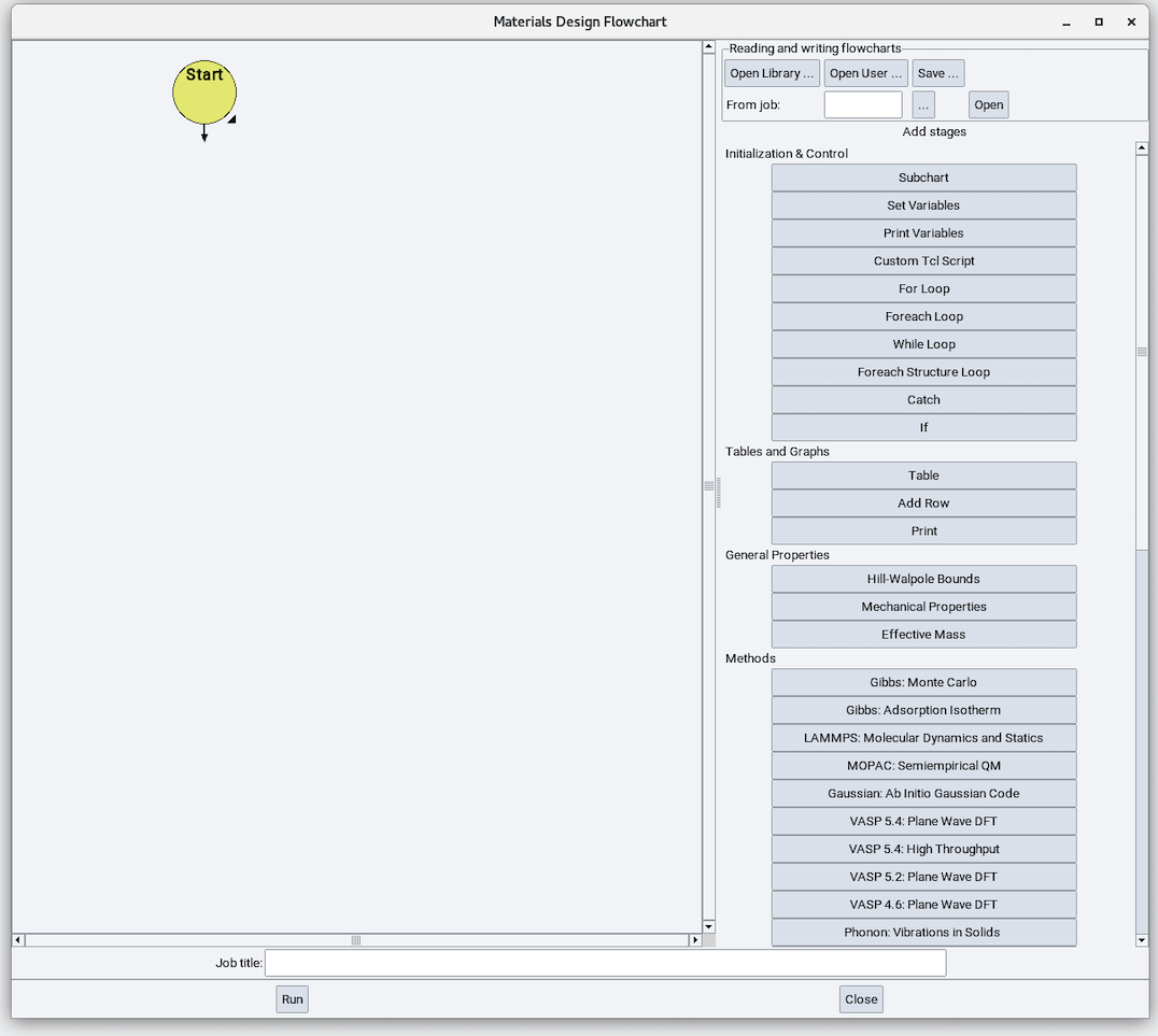
2.20.2. Variables

A MedeA LAMMPS flowchart usually starts with a Variables stage:

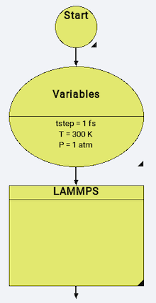
With simulation variables defined in the following way:

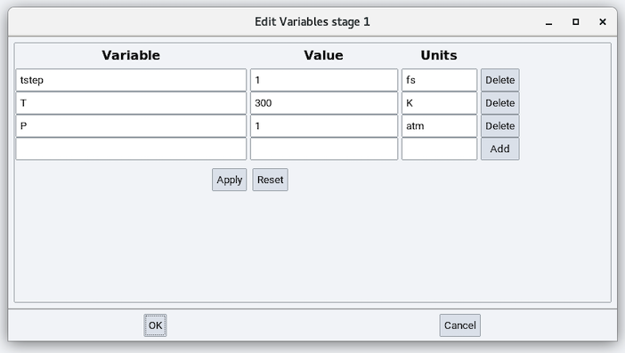
If no simulation variables are defined, the LAMMPS stages use the following default variables:

• Time step (tstep): 1 fs
• Temperature (T): 300 K
• Pressure (P): 1 atm

2.20.3. Initialization

On opening the LAMMPS stage you will see a LAMMPS flowchart:

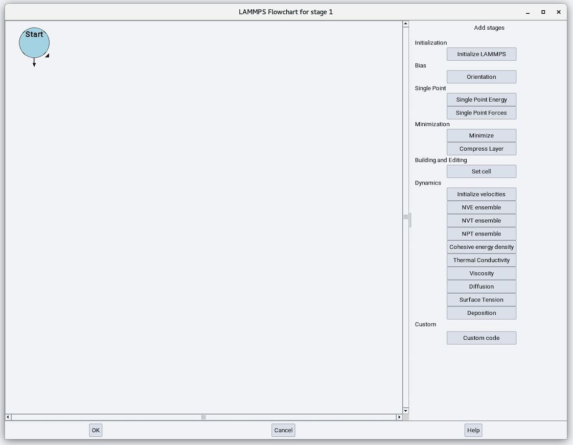
The Initialization section from the right-side panel has one available stage: Initialize LAMMPS. The LAMMPS stage starts with the Initialize stage:

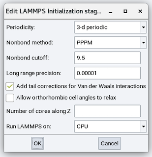
The parameters are:

• Periodicity: Choose from 3-d periodic for bulk systems and layer perpendicular to Z for slab models.

  Hint

  Even with 3-D periodic boundary condition, a slab model can be created by having large enough vacuum size (> ~15 \({\mathring{\mathrm{A}}}\))

• Nonbond method: For long-range Coulombics, choose from Cutoff for a simple spherical cutoff, PPPM for particle-particle/particle-mesh Ewald, and Ewald for conventional Ewald.

• Nonbond cutoff: Cutoff value for spherical or real-space cutoff. The default value of 9.5 is usually good.

• Long range precision: Only used with PPPM and Ewald methods. Determines the reciprocal-space convergence. The default value of 0.00001 is usually a good value.

• Add tail corrections for Van der Waals interactions: The default is yes.

• Allow orthorhombic cell angles to relax: Check this box if you have an orthorhombic cell but you also would like to relax all 6 cell parameters including a, b, c, alpha, beta, and gamma. The default is no.

• Number of cores along Z: For slab models where there is a large vacuum space, it is usually faster and more robust to use only 1 core along the plane normal direction. To use this feature, align the plane normal along the Z direction and enter 1.

• Run LAMMPS on: Choose from CPU or GPU.

  Note

  MedeA LAMMPS supports LAMMPS on Nvidia Tesla series GPUs.

2.20.4. Bias

The Bias section has one available stage: Orientation:

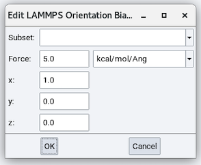
The parameters are:

• Subset: Add bias to this atom pair subset.
• Force: magnitude of the added bias.
• x, y, and z: direction of the added bias.

2.20.5. Single Point

The Single Point section has two available stages: Single Point Energy and Single Point Forces. Both of these stages have no adjustable parameters.

2.20.6. Minimization

The Minimization section has two available stages: Minimize and Compress Layer.

2.20.6.1. Minimize

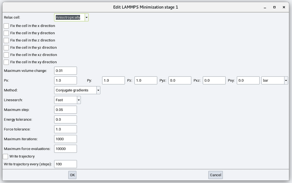
The Minimize stage has the following parameters:

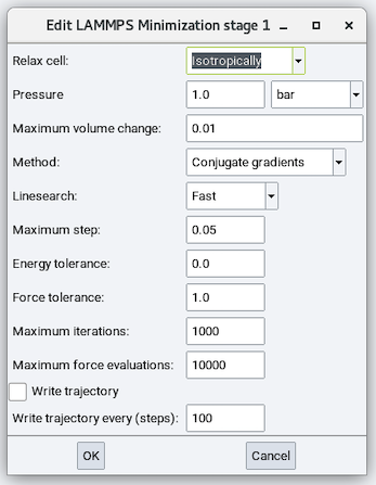
• Relax cell: Choose from No, Isotropically, With x=y, With y=z, With x=z, and Anisotropically and depending on the choice, there are zero to six cell parameters to fix (remain unchanged during minimization), zero to six stress values to relax each cell parameter to, and maximum volume change:

  

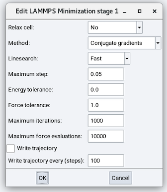
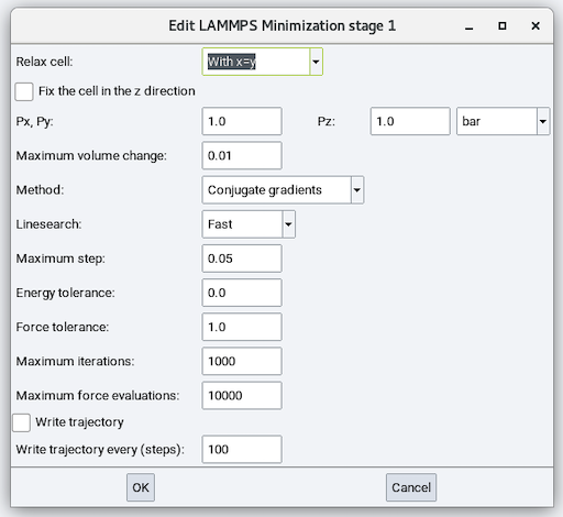
• Method: Choose from Conjugate Gradient (CG), Steepest Descent (SD), and Hessian-free truncated Newton (HFTN). The default is CG.

  CG method is the Polak-Ribiere version. At each iteration, the force gradient is combined with the previous iteration information to compute a new search direction perpendicular (conjugate) to the previous search direction. The PR variant affects how the direction is chosen and how the CG method is restarted when it ceases to make progress. The PR variant is thought to be the most effective CG choice for most problems.

  With the SD method, at each iteration, the search direction is set to the downhill direction corresponding to the force vector (negative gradient of energy). Typically, steepest descent will not converge as quickly as CG, but may be more robust in some situations.

  With the HFTN algorithm, at each iteration, a quadratic model of the energy potential is solved by a conjugate gradient inner iteration. The Hessian (second derivatives) of the energy is not formed directly but approximated in each conjugate search direction by a finite difference directional derivative. When close to an energy minimum, the algorithm behaves like a Newton method and exhibits a quadratic convergence rate to high accuracy. In most cases the behavior of HFTN is similar to CG, but it offers an alternative if CG seems to perform poorly.

  Warning

  When changing cell parameters, only the conjugate gradient and steepest descent methods can be used.

• Linesearch: Choose from Fast, Quadratic, or Backtrack. The default is Fast.

• Maximum step: Maximum distance (\({\mathring{\mathrm{A}}}\)) to move atoms. The default value of 0.05 is usually good.

• Energy tolerance: The default is 0.0 eV or Kcal/mol.

• Force tolerance: The default is 1.0 eV/\({\mathring{\mathrm{A}}}\) for metallic/NIST and COMB3 forcefields and 1.0 Kcal/mole-\({\mathring{\mathrm{A}}}\) for all other forcefields.

• Maximum iterations: Maximum iterations for energy evaluations. The default is 1000.

• Maximum force evaluations: Maximum iterations for force evaluations. The default is 10000.

• Write trajectory and the required value for Write trajectory every (steps): 100.

2.20.6.2. Compress Layer

The Compress Layer stage does not relax cell parameters but compresses the materials in the simulation cell. It is similar to the Minimize stage with the following exceptions:

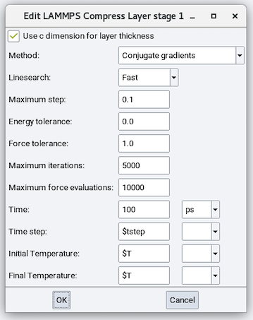
• Use c dimension for layer thickness: Check this box to have the final c cell parameter unchanged or uncheck this box to define a final c cell parameter.
• Time: Simulation time.
• Time step: time step size for NVT integration.
• Initial Temperature and Final Temperature: Initial and final temperature for NVT integration.

Warning

A Compress Layer stage must be used with layer perpendicular to Z periodicity and Cutoff Nonbond method.

2.20.7. Building and Editing

This section has one available stage: Set cell:

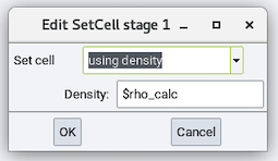
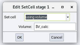
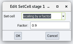
• Set cell: Changes the cell dimension by one of the following
  • using density and its Density
  • using volume and its Volume
  • scaling by a factor and its Factor

All of the above options can be a value or a variable.

2.20.8. Dynamics

The Dynamics section has ten stages and the following stages are included in MedeA LAMMPS license:

• Initialize velocities
• NVE ensemble
• NVT ensemble
• NPT ensemble

While the following stages (modules) require additional licenses:

• Cohesive energy density
• Thermal Conductivity
• Viscosity
• Diffusion
• Surface Tension
• MedeA Deposition

2.20.8.1. Initialize Velocities

The Initialize velocities stage thermalizes the cell to a user-defined temperature:

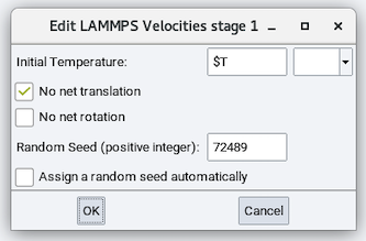
• Initial Temperature: temperature to thermalize the cell to
• No net translation: Whether to randomize thermal velocities so no net translation exists.
• No net rotation: Whether to randomize thermal velocities so no net rotation exists.
• Random Seed (positive integer): A random seed for the random number generator. It can be assigned manually.
• Assign a random seed automatically: randomly generates a random seed.

2.20.8.2. NVE ensemble

The NVE stage performs time integration without the equations of motion altered.

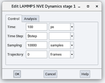
The parameters in the Control tab are:

• Time: Duration of the simulation run (defaults to 100 ps).
• Time Step: Time step size employed in solving the equations of motion.
• Sampling: Number of samples employed in performing averaging. This parameter does not affect dynamics.
• Trajectory: Number of trajectory frames saved during the molecular dynamics calculation. This parameter does not affect dynamics.

The Analysis tab allows you to add Distance analysis and Distribution analysis. The Distance Analysis analyzes the interatomic distance between pairs of atoms defined by a pair subset, while the Distribution Analysis analyzes the spatial distribution of the given subset.

Warning

Using an NVE stage does not automatically guarantee an NVE ensemble. You should examine Job.out and the energy profile to ensure that the total energy is conserved so that an NVE ensemble is achieved.

2.20.8.3. NVT ensemble

The NVT stage performs time integration with a thermostat added to the equations of motion.

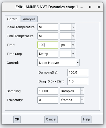
The parameters in addition to those in the NVE stage are:

• Initial Temperature and Final Temperature: These two parameters can be the same or different (for establishing a cooling or heating). These parameters can be values or variables.

• Control: Choose a thermostat algorithm from one of the following:

  rescaling: interval (steps), window, amount of rescaling

  Langevin: Damping (fs), Random Seed (integer)

  Berendsen: Damping (fs)

  Nose-Hoover: Damping (fs) and Drag

  Hint

  The default option of Nose-Hoover and Langevin are the best choices for a thermostat. The Damping parameter is recommended to be 100 times the time step size. For example, for a 1 fs time step, the Damping is recommended to be 100 while for a 0.2 fs time step its recommended value is 20.

Warning

Using an NVT stage does not automatically guarantee an NVT ensemble. You should examine Job.out and the temperature profile to ensure that temperature is maintained at the defined value so that an NVT ensemble is achieved.

2.20.8.4. NPT ensemble

The NPT stage performs time integration with a thermostat and a barostat add to the equations of motion.

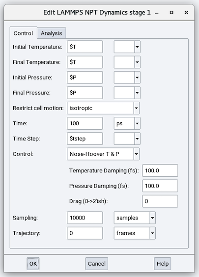
The parameters in addition to those in the NVT stage are:

• Initial Pressure and Final Pressure: These two parameters can be the same or different (for establishing a shrinkage or an expansion). These parameters can be values or variables.

• Restrict cell motion: Controls how the cell volume and shape are equilibrated/relaxed:

  • isotropic: Only a, b, and c cell parameters (x, y, and z dimensions) are relaxed and the three components relax to one averaged value.

  • fixed angles: Also known as anisotropic with a, b, and c cell parameters relaxed independently

  • constrained: Allows users to choose to relax any of the six cell parameters (a, b, c, alpha, beta, and gamma) independently.

  • unconstrained: All six cell parameters relax independently.

    Warning

    To relax the cell with constrained or unconstrained options, the cell must be non-orthorhombic or you need to check the box Allow orthorhombic cell angles to relax in the Initialize state.

• Control: Choose a combination of thermostat and barostat from the following options:

  Rescaling/Berendsen: Interval (steps), Window, Amount of rescaling, Pressure Damping (fs), Bulk modulus

  Langevin/Berendsen: Damping (fs), Random Seed (integer), Bulk modulus

  Berendsen/Berendsen: Damping (fs), Pressure Damping (fs), Bulk modulus

  Nose-Hoover T/Berendsen: Damping (fs), Drag (integer), Pressure Damping (fs), Bulk modulus

  Nose-Hoover T & P: Temperature Damping (fs), Pressure Damping (fs) and Drag (0 to 2’ish)

  Hint

  The default option of Nose-Hoover T & P is the recommended combination of thermostat and barostat

Warning

Using an NPT stage does not automatically guarantee an NPT ensemble. You should examine Job.out and the temperature, stresses, and pressure profiles to ensure that temperature, stresses, and pressure are maintained at the defined value so that an NPT ensemble is achieved.

2.20.8.5. Cohesive energy density

The Cohesive energy density stage is a separate module available from Materials Design. It performs time integration under an NVT ensemble while making automated extractions and calculations to calculate the cohesive energy density.

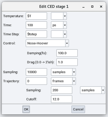
The parameters in addition to those in the NVT stage are:

• CED Sampling: Calculate cohesive energy density every this many steps.
• CED Cutoff: The Cutoff value to calculate the energy.

Results are written in Job.out.

2.20.8.6. Thermal Conductivity

The Thermal Conductivity stage is a separate module available from Materials Design and described in section Thermal Conductivity

2.20.8.7. Viscosity

The Viscosity stage is a separate module available from Materials Design and described in section Viscosity

2.20.8.8. Diffusion

The Diffusion stage is a separate module available from Materials Design and described in section Diffusion

2.20.8.9. Surface Tension

The Surface Tension stage is a separate module available from Materials Design. It performs time integration under an NVT ensemble while calculating the surface tension. It has the same parameters from the NVT stage.

2.20.8.10. Deposition

Is a separate module available from Materials Design and described in Section MedeA Deposition

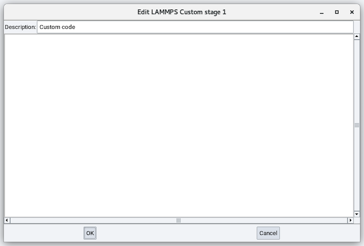
2.20.9. Custom

The Custom stage is available with MedeA LAMMPS license. It enables the addition of any custom LAMMPS commands not accessible from the above stages. Variables defined in any previous stages are passed into the Custom stage.

2.20.10. Example

This flowchart illustrates the efficient use of MedeA LAMMPS flowchart:

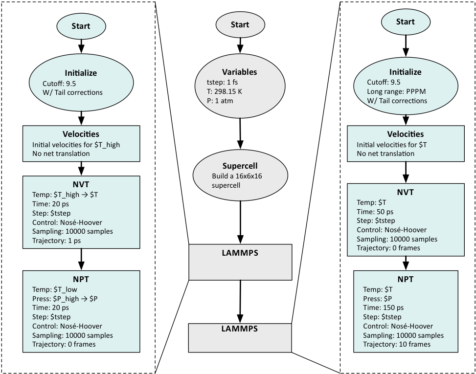
The Variables stage defines the overall parameters for temperature, pressure and basic time step.

A larger supercell is constructed from the provided molecule.

Two different LAMMPS stages can be required, when the first equilibration stage makes use of a computationally less demanding approach for non-bond interactions (e.g. Cutoff) for simple equilibration.

The most accurate energy calculations and sampling (for some type of molecules) requires Ewald summation or PPPM and occurs in the second LAMMPS stage.

download:pdf