2.1. MedeA Overview

---

download:pdf

---

2.1.1. MedeA modules at a glance

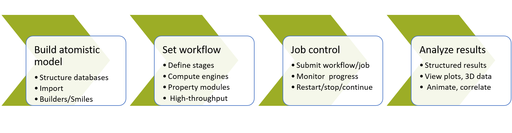
The MedeA graphical simulation environment includes experimental databases and tools/modules for computing chemical and physical materials properties based on atomistic models, with a great level of automation.

A typical MedeA workflow may involve a database search for experimental structure information and/or a building step to refine or modify a structure model, followed by one or several compute stages, including post-processing for predicting materials properties such as structure, energetics, dynamics or other derived information.

In the following, we describe MedeA functionality by:

• modules, and
• materials properties.

MedeA modules at a glance

• The MedeA environment, often referred to as MedeA GUI, is comprising a graphical workspace with base modules for structure handling, job submission and monitoring as well as analysis tools. The documentation section Performing Computations with MedeA describes how to get started with the environment.
• MedeA InfoMaticA for searching and retrieving structure models from experimental structure databases and handling user-generated data. MedeA’s experimental databases include
  • COD (Crystallography Open Database, University of Cambridge, UK)
  • ICSD (Inorganic Crystal Structure Database, FIZ Karlsruhe, Germany)
  • NCD (NIST Crystal Data, National Institute of Standards and Technology, USA)
  • Pearson’s File (ASM International, USA)
  • The Linus Pauling file (LPF), binary edition (MPDS, Switzerland)
• MedeA tools for Building and Structure Editing of crystalline systems and molecules
• MedeA Special Builders for supercells and surfaces, defects in structures and nanoparticles, as well as fluids, polymers, amorphous systems and thermosets. MedeA special builders also include a stack layer builder, a docking tool and a GUI for setting up heterogeneous interfaces and grain boundaries.
• MedeA Flowcharts to set up workflows and compute jobs or to load pre-built workflows from the jobserver, the workflow library or external sources.
• MedeA compute engines for electronic structure calculations
  • MedeA VASP 5.4
  • MedeA Gaussian
  • MOPAC 2009/2012/2016
• MedeA compute engines for classical, forcefield based calculations
  • MedeA GIBBS - Monte Carlo calculations for fluids and for adsorption of fluids in solids (statistical ensembles: NVT, NPT, osmotic, GEMC, GCMC)
  • MedeA LAMMPS - Molecular dynamics simulations using classical and reactive forcefields (statistical ensembles: NVT, NPT, NVE)
• MedeA tools for Analysis of Results including structure/geometry/symmetry analysis, electronic structure, trajectories and Automated Convergence analysis
• MedeA property modules use MedeA engines to automate property calculations. These Property modules include
  • MedeA Diffusion
  • MedeA Viscosity
  • MedeA Thermal Conductivity
  • MedeA Deposition
  • MedeA MT - Elastic Properties
  • MedeA Phonon
  • MedeA UNCLE
  • MedeA Electronics
  • MedeA Transition State Search
• The MedeA Forcefields package includes many forcefield parameter sets, of both non-reactive and reactive forcefields, for organic and inorganic materials, metals, semiconductors; all forcefields can be viewed and edited
• MedeA Forcefield Optimizer combines quantum mechanical and classical simualations to optimize and validate forcefield parameters
• MedeA HT provides a powerful framework for high-throughput (HT) calculations
• MedeA QT is a general toolkit for QSPR analysis
• MedeA P3C deploys topological descriptors
• MedeA QSPR uses the Joback group contribution method to predict thermophysical properties of organics

2.1.2. MedeA capabilities by materials property

The MedeA environment is designed to give quick access to materials property data both by mining experimental data and by computing properties where experimental data is scarce or only partly available. MedeA includes graphical user interfaces to accomplish search and retrieval of experimental data, structure building, setup of computations and data visualization and analysis.

Given the rapid progress with sub-micron and even nanoscale devices, and the increase in technical and environmental demands on materials and processes, decisive experiments are often time consuming and expensive. Computations can help to prepare, design and interpret experiments.

However, just like performing a complex experiment, setting up computations requires scientific and technical rigor, precision and careful analysis. MedeA helps you to achieve these qualities by:

• Providing experimental data as starting points for computations
• Giving access to industrially qualified routines for structure analysis and structure building
• Using high-end computational codes with a complete set of defaults and convergence tests
• Automating complex multi-step calculations
• Enabling you to run thousands of calculations using a powerful job management and data processing paradigm

In the following, we provide a short overview of key properties and related modules:

Individual MedeA functionality is highlighted.

MedeA capabilities by materials property

• Experimental structure, powder pattern, neutron diffraction data
• Search & Retrieve lattice parameters atomic positions and related data from structure databases COD, ICSD, Pauling, Pearsons and NIST using InfoMaticA
• Build crystal structures, surfaces and molecules using MedeA’s Builders
• Analyze structures for symmetry, bonds and angles, visualize empty space, plot nearest neighbors and powder pattern using Geometry Analysis and Empty Space Finder
• Thermodynamic stability, elastic constant, elastic modulus
• Compute energies of formation using VASP , MOPAC or Gaussian
• Compute the temperature dependence of formation energies using PHONON or MT in combination with VASP or LAMMPS
• Fully automated strain-stress analysis to derive elastic constants using MT in combination with VASP or LAMMPS
• Substitutional and interstitial defects, defect insertion energies
• Study substitutional defects using Substitutional Search
• Find empty space and determine the coordination of interstitial sites using Empty Space Finder
• Vibrational spectroscopy, thermodynamics, diffusion
• Raman/Infrared data
• Use PHONON or MOPAC to get the positions of RAMAN/IR peaks from the full PHONON spectrum
• In PHONON, graphically visualize, characterize and animate lattice vibrational modes and PHONON density of states
• Thermodynamic functions, phase stability
• Compute the Free energy, vibrational entropy and specific heat as a function of Temperature using PHONON
• Segregation, diffusion barriers
• Compute bulk/surface and bulk/interface segregation energies using VASP
• Find transition states and diffusion barriers using Transition State Search
• Get temperature dependence using PHONON
• Fluid phases, Vapor-Liquid Equilibria
• Compute single phase properties: pressure, density, composition, configuration enthalpy, residual heat capacity, speed of sound, thermal expansion, isothermal compressibility of a single liquid or gas phase. Also, estimate the chemical potential of a molecular species and Henry solubility constants of a gas in a liquid using GIBBS. Compute density, enthalpy, cohesive energy density, viscosity, thermal conductivity and surface tension of a fluid phase using LAMMPS. Compute self-diffusivity of a species in a fluid, using LAMMPS.
• Compute phase equilibria properties: pressure, density, composition, vaporization enthalpy / normal boiling point / critical point (pure compounds) and equilibrium constants (mixtures) using GIBBS
• Adsorption in solids, surface adsorption
• Compute sorption isotherms using GIBBS of gases in zeolites, MOF’s, ZIF’s, polymers
• Determine adsorption geometries, binding energies and bond frequencies of molecules on surfaces using PHONON and VASP

2.1.3. MedeA capabilities by computational approach

2.1.3.1. Electronic structure methods

At the most fundamental level, MedeA computes the electronic structure of materials from quantum mechanics, thus providing interatomic forces, molecular and crystal structure and chemical information such as formation energies or binding energies. Relevant MedeA electronic structure engines are VASP, GAUSSIAN and MOPAC.

2.1.3.2. Forcefield based Molecular Dynamics and Monte Carlo

Physical interactions involving many atoms or molecules are most efficiently described by inter-atomic potentials or so-called force fields. Relevant MedeA engines making use of forcefields are the classical molecular dynamics code LAMMPS and the Gibbs Ensemble Monte Carlo code GIBBS.

2.1.3.3. Coarse grain potentials

Unifying interatomic potentials reduces the number of effective particles in a system, and thus let’s you deal with larger systems and longer simulation times. Both LAMMPS and GIBBS support several types of coarse grain potentials.

2.1.3.4. Configurational disorder

Decomposing a periodic systems with the configurational disorder (alloys, vacancies, defects) into clusters, the MedeA Universal Cluster Expansion code UNCLE addresses systems with up to millions of atoms. UNCLE uses VASP or LAMMPS to compute individual cluster contributions.

2.1.3.5. Correlations, QSAR, group addition

MedeA also offers a number of statistical methods to create correlations between experimental or computed descriptor data: P3C uses molecular-level topological data (Bizerano-method), the Joback method exploits the additivity of certain group properties and MedeA QT lets you create general correlations for any data of input data.

2.1.3.6. Property Prediction Modules

Property calculations often involve repeated systematic use of QM/MD/MC compute engines on many dozens or hundreds of input systems, yielding quantities like mechanical and thermal properties, vibrational properties, thermodynamic functions, reaction energies, transport properties, etc.

MedeA offers fail-safe automation in preparing, executing and post-processing compute jobs through its property modules wherever computational protocols can be sufficiently standardized. Examples are Universal Cluster Expansion for alloys with UNCLE, Fluid Adsorption Isotherms with GIBBS or the prediction of Viscosity and Thermal conductivity from Green-Kubo theory or Non-Equilibrium Molecular Dynamics with MedeA Viscosity and MedeA Thermal Conductivity.

The following tables provide a non-exhaustive list of materials properties which can be addressed with MedeA.

2.1.3.7. Examples of solid-state properties

Structural Properties	Thermo-mechanical Properties	Thermodynamic Properties
Lattice parameters	Density, elastic moduli, speed of sounds	Heats of formation, Free energy, \(\Delta H, \Delta U, \Delta S, \Delta G, c_v\)
Bond lengths and bond angles	Thermal expansion	Binding energies, miscibility
Adsorption geoemtries, interface gaps	Fracture	Vapor pressure, surface tension

2.1.3.8. Examples of solid-state properties

Chemical Properties	Transport Properties	Electronic, optical, magnetic
Heat of reaction	Mass diffusion coefficients	Electronic density of states and dispersion, molecular orbitals
Activation energies	Thermal/electronic conductivity	Spin, band gap, work functions

2.1.3.9. Examples of fluid-state properties

Chemical Properties	Transport Properties	Thermodynamic Properties
Ideal gas capacity \((c_{p,id})\)	Self diffusivity \((D)\)	Critical Point \((T_c, P_c, V_c)\)
Dipole moment \((\mu)\)	Viscosity \((\eta)\)	Vaporization enthalpy \((\Delta H_{vap})\)
Quadrupole moment \(Q\)	Thermal conductivity \((\lambda)\)	Normal boiling point \((T_b)\)
Polarizability \(\alpha\)		Saturation pressure \((P_{sat})\)
Ideal gas Heat of Formation \((\Delta G_{f})\)		Water solubility, w/o partition coefficient
Ideal gas Gibbs Energy of Formation \((\Delta G_{f})\)		Residual heat capacity \((c_{p,res})\)
Lower Heat of Combustion \(PCI\)		Joule Thomson coefficient \((\mu_{JT})\)
Upper Heat of Combustion \(PCS\)		Speed of spound \((U_s)\)
Electronegativity \((\chi)\)		acentric factor \((\omega)\)

download:pdf