2.21. Thermal Conductivity

---

download:pdf

---

Key Benefits of MedeA Thermal Conductivity

• Automatic analysis including fitting of results
• Quick and easy validation based on graphs, reported fitting errors and access to all intermediate results through the convenient web interface
• Integrated with MedeA Forcefield for advanced forcefield handling and assignment

Note

Generally there are two contributions to the thermal conductivity of a material as follows:

• Electronic contribution: depends on the electronic band structure, electron scattering, and electron-phonon interaction.
• Lattice contribution: depends mainly on the phonons (nuclear vibrations) and phonon scattering.

MedeA Thermal Conductivity calculates the lattice contribution to the thermal conductivity using forcefield methods. When necessary, you may also use MedeA VASP and MedeA Electronics to calculate the electronic contribution.

2.21.1. Equilibrium Molecular Dynamics (EMD)

This is also known as the Green-Kubo Method, which calculates thermal conductivity from the integral of the autocorrelation function of the heat flux. It is only applicable for homogeneous configurations, i.e., no defects, interfaces, multiple phases, etc. The required length of the simulation depends on the thermal conductivity, with higher conductivities requiring longer simulation times. It provides reasonable approximations for systems with small atomic charges, such as hydrocarbons, many semiconductor alloys, etc. A significant advantage is that it requires only moderate system sizes.

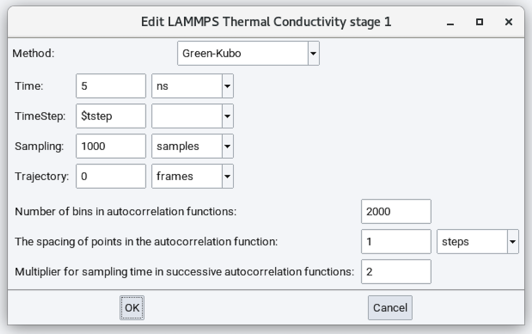
• Method: Green-Kubo
• Time: Duration of the simulation run (defaults to 5 ns).
• Time Step: Time step size employed in solving the equations of motion.
• Sampling: Number of samples employed in performing averaging. This parameter does not affect dynamics.
• Trajectory: Number of trajectory frames saved during the molecular dynamics calculation. This parameter does not affect dynamics.
• Number of bins in autocorrelation function: 2000
• The spacing of points in the autocorrelation function: 1 step
• Multiplier for sampling time in successive autocorrelation functions: 2

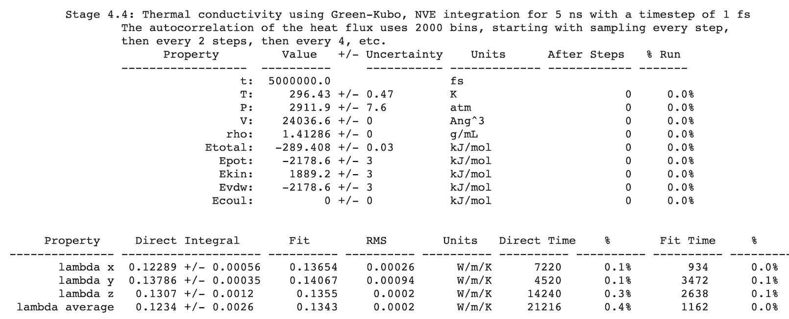
After completing a simulation, results are written to Job.out. For example:

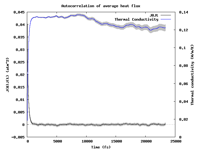
Additionally, visualization of the autocorrelation function and its integral, the thermal conductivity, are available as {stage_id}_JJt_decay_average.gif. For example:

Hint

If you would also like to calculate viscosity from the autocorrelation function of stress tensor using the Green-Kubo algorithm and you have a license for MedeA Viscosity, you can use a checkbox in the Viscosity stage to calculate both the thermal conductivity and viscosity:

Also calculate thermal conductivity

This option reduces computational expense when you would like to calculate both the viscosity and thermal conductivity in one stage!

2.21.2. Reverse non-equilibrium molecular dynamics method (RNEMD)

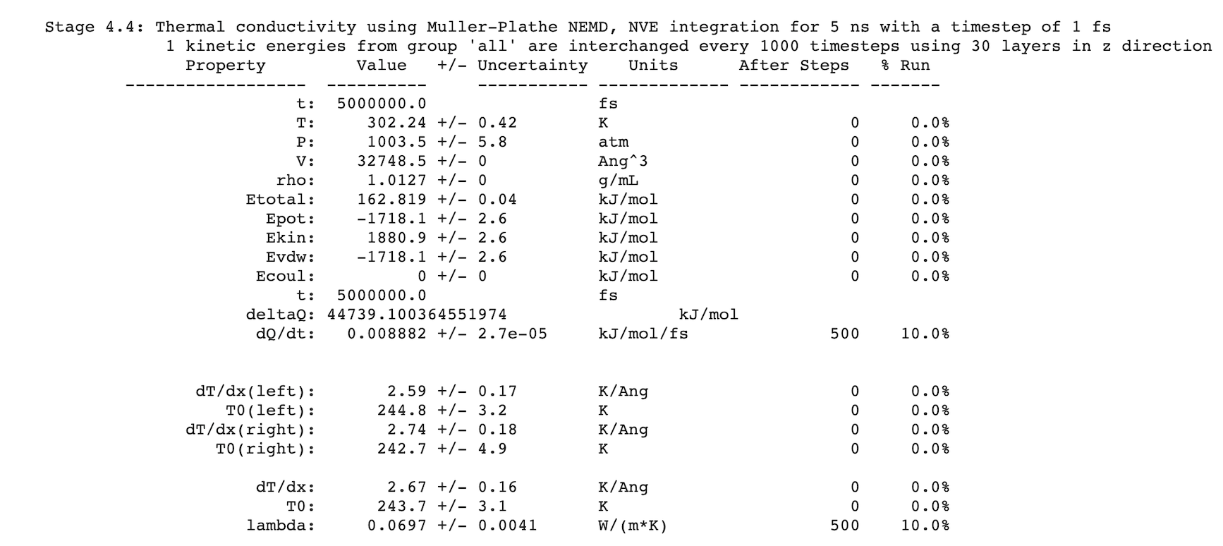
This is also known as the Müller-Plathe [1] method, which induces a temperature gradient (heat flux) by performing kinetic energy swaps between atoms in hot and cold regions, and monitors the resulting temperature profile. Thermal conductivity is calculated as the ratio of the heat flux to the slope of the temperature profile. The method applies to all systems but requires elongated cells in the direction of heat transfer. Higher conductivities, which arise from longer phonon mean free path lengths, require correspondingly longer cells. The effect of the cell cross-section should ideally be examined, and heat transfer rate (flux) may need to be optimized, requiring some user intervention.

The different parameters are:

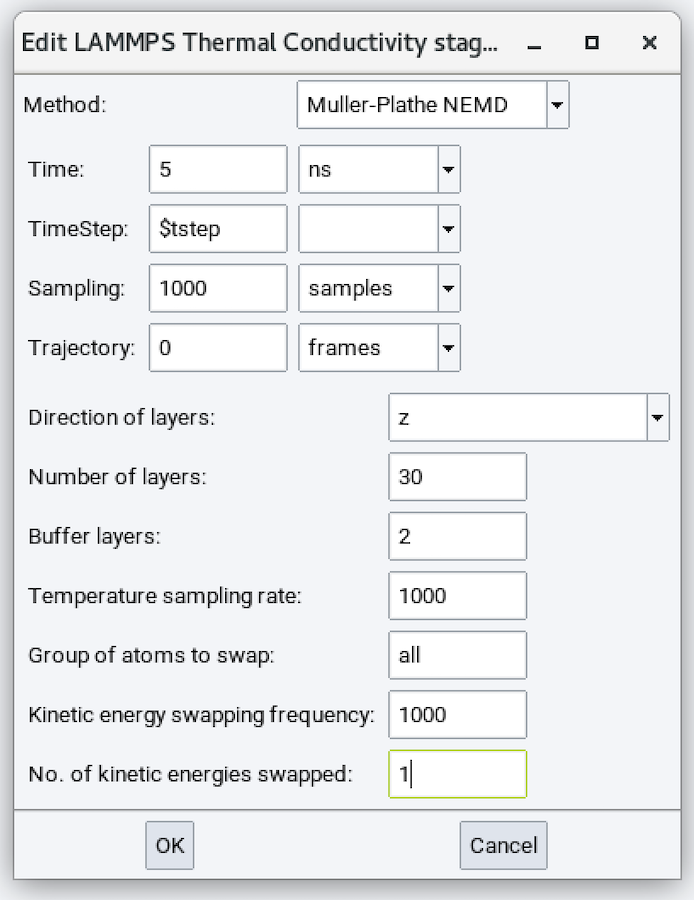
• Method: Muller-Plathe NEMD
• Direction of layers: Direction in which the temperature gradient should be established.
• Number of layers: Divides the above direction into this many layers to calculate the temperature profile.
• Buffer layers: Number of layers on and near the boundary that are not used in the final analysis.
• Temperature scaling rate: Sample kinetic energy every this many steps. The default value of 1000 can usually be accepted.
• Group of atoms to swap: Defaults to all.
• Kinetic energy swapping frequency: Defaults to 1000.
• No. of kinetic energies swapped: Defaults to 1.

After completing a simulation, results are written to Job.out. For example:

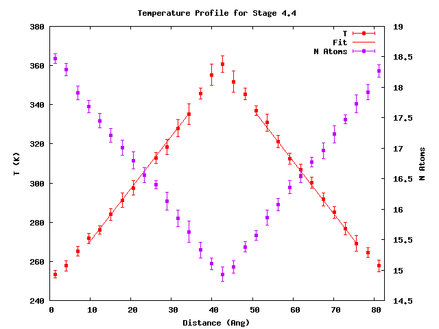
Additionally, visualization of the temperature profiles is available as {stage_id}_average_temperature_profile.png. For example:

[1]	Florian Müller-Plathe and Dirk Reith, “Cause and Effect Reversed in Non-Equilibrium Molecular Dynamics: an Easy Route to Transport Coefficients”, Computational and Theoretical Polymer Science 9, no. 3 (1999): 203-209.

download:pdf