2.17. Transition State Search
Contents
| download: | pdf |
|---|
The Transition State Search module combines different computational approaches to find the minimum energy pathway between an initial and a final atomic configuration, and to search and refine transition states within this minimum energy path, in a given direction or in randomly chosen directions. For mapping out the minimum energy path it uses a chain of configurations (called images) connected by elastic springs, calculates forces for each configuration and uses information from neighboring images to optimize all configurations in the chain (Nudged Elastic Band Method). At each of the energy maxima along the path, transition states can be searched for, refined and optimized by elastic band methods, by means of so-called mode following techniques (Dimer Method) and energy based optimization techniques (RMM-DIIS).
The overall goal is to find one or more saddle points of the energy hypersurface, whose configuration has a local energy minimum in all but one coordinate. That can be verified by looking at their phononic or vibrational spectrum, which has one imaginary frequency in such a case.
This module combines several methods to map out the minimum energy path and attempts the optimization of transition states. Based on the JobServer/TaskServer architecture, transition state search may run on any hardware configuration from single processor desktop machines up to highly parallel computer racks.
2.17.1. Basic Tasks
Select Tools >> Transition State Search to access a new item appearing in the menu bar. Click on Transition State Search to open the menu. The menu’s first section displays three different tasks:
Map the reaction path and find transition states brings up a panel to configure an optimization of the minimum energy path between initial and final state followed by a search and optimization of transition states along the path.
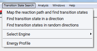
Find transition state in a direction brings up a panel to configure transition state search and optimization starting from the initial state in a direction towards another state by means of the Dimer Method.
Find transition states in random directions brings up a panel to configure transition state search and optimization in a number of different randomly chosen directions by means of the Dimer Method.
Furthermore, Select Engine allows for selecting a specific VASP version. The three tasks above are only supported by VASP 5.3. For VASP 5.2 and 4.6 a restricted set of simulation options are available from a different user interface (not shown here).
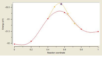
Energy Profile visualizes and analyzes the energy and structures along the path between the initial and final image, which is created by running the task Map the reaction path and find transition states. In the example above, there are 4 images (denoted by red points) between the initial and final image, defining the values 0 and 1 of the reaction coordinate. One refinement step between images 2 and 4 created the finer orange mesh of images. In a further step, the transition state is refined by means of the Dimer Method (not resolved in the graph). Finally, an optimization of the transition state leads to the configuration marked by the blue diamond. The basic workflow of this task and its computational options are described below, the output and analysis of results are presented in Section Output for Reaction Path Mapping. The other two tasks related to the Dimer Method are discussed in sections Find Transition State in a Direction and Find Transition States in Random Directions.
2.17.2. Map the Reaction Path and Find Transition States
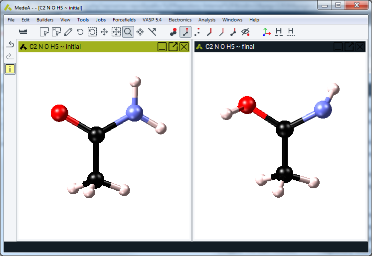
2.17.2.1. Select Initial Configuration
Select the structure window with the initial configuration and make it active, so that its title bar turns blue. The initial configuration must be a periodic model of symmetry P1 (no symmetry defined).
Note
If some atoms of the selected initial configuration are frozen, these degrees of freedom are omitted from the optimization process. As a consequence these atoms are not moved and remain fixed for all images.
Click on Transition State Search >> Map the reaction path and find transition states to select the final configuration and to configure the protocol for the minimum energy path and transition state search and optimization.
2.17.2.2. Select Final Configuration
All periodic structure windows with a matching configuration (identical stoichiometry and cell contents) and P1 symmetry are available for being selected as the final configuration. Click on the button next to the final configuration to change the proposed choice.

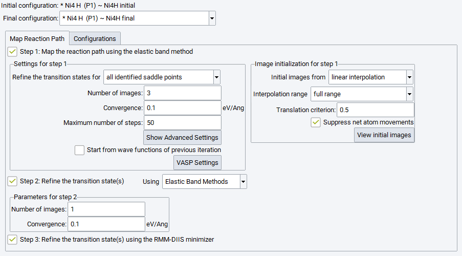
2.17.2.3. Step 1: Map the Reaction Path Using the Elastic Band Method
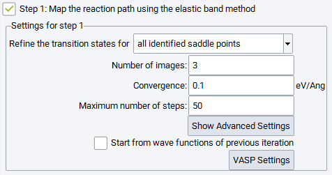
The first step of this simulation protocol is mandatory and cannot be deselected. Its objective is to explore the energy hypersurface and to identify possible locations of transition states and intermediate minima along the reaction pathway. In the subsequent steps, such candidates for transition states can be refined and optimized either for all identified saddle points or for the highest saddle point only. Three main parameters define the mapping of the reaction path by means of elastic band methods:
Number of images: The number of images needed depends on the complexity of the reaction path (single or multiple saddle points), the reaction barrier and the distance between respective atoms in the initial and final image. A smaller number of images can still deliver excellent energy barriers when using refinement steps or the climbing image option (see the Advanced Settings below).
Convergence: sets the criterion for stopping the optimization process, also for refinement steps. The maximum force acting on any atom of any image including the spring contributions is tested.
Maximum number of steps allowed for the optimization process, also for each refinement step
Pushing the Show Advanced Settings button displays a number of further options to trigger the performance of the elastic band technique:
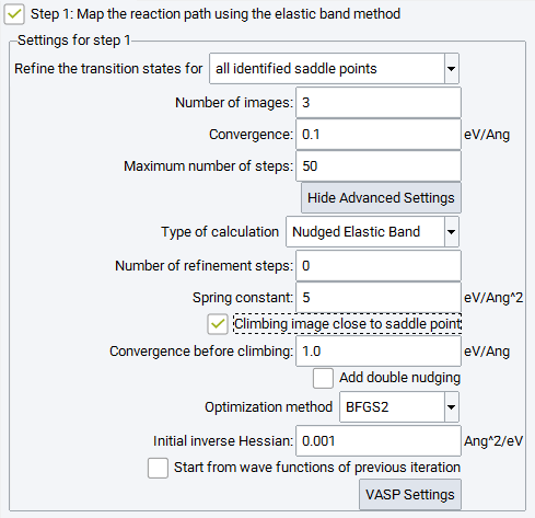
For the Type of calculation there is a choice between two variants of the Elastic Band method: Nudged Elastic Band or Elastic Band. For the conceptual difference between these approaches see the methodological section.
The Number of refinement steps after the initial elastic band calculation is finished, a refinement step sets up the same number of linearly interpolated images between two images bracketing the expected saddle point. With a small number of images the transition barrier can be over or underestimated; creating a finer distance between the images by increasing their number also increases the computational cost and affects convergence. Refinement overcomes this situation by a closer examination of the region around the suspected transition states.
Spring constant: Atoms of adjacent images are connected by elastic springs to keep images close to the minimum energy path. The spring constant determines the chain stiffness. A soft chain allows adjacent images to differ substantially from each other and may sample a larger search space, however, it is more vulnerable to corner cutting and down sliding of images in steep and curved sections of the energy hypersurface. The recommended default value is 5 eV|AA|2.
Initial inverse Hessian matrix: the diagonal elements are set to this value and condition the optimizer to take bold moves or rather small steps.
Reduce the value of the initial inverse Hessian, if the initial gradient is too big and the chain of images gets off track after 3 or 5 steps. A general value for all systems cannot be provided, as the choice depends on the ratio of moving atoms to more or less static atoms, initial forces and masses of moving atoms.
Additional options specific for the nudged elastic band method are:
Climbing image close to the saddle point: The almost equidistant images of a nudged elastic band may be inconveniently aligned off the saddle point positions. As an alternative to refinement steps, a selected image close to the saddle point can be made climbing up into the transition state, once the convergence reaches a value specified by Convergence before climbing. This may yield transition states directly by a single optimization without an intermediate second step for further refinement.
Add double nudging: This uses a refined scheme for calculating the forces perpendicular to the chain of spring connected images (see methodological section). Depending on the energy hypersurface, this can improve the convergence process.
2.17.2.4. Image Initialization
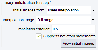
As a default, initial images are obtained from linear interpolation, i.e. without user interaction a set of linearly interpolated images will be used to create the initial chain between the initial and final configuration filling the full range.
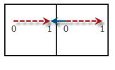
Translation criterion deals with some ambiguity in setting up the initial chain of images due to the periodicity of the cell: When the distance between matching atoms in the initial and final configuration is larger than half of the respective cell coordinate, the movement can be either within the cell or between the atom and its periodic copy in a neighboring cell.
The value of 0.5 always uses the shortest distance between the initial and final image, whereas a larger value allows for longer paths within the cell. In the illustration on the right, a value of 0.75 is needed to allow for the path indicated by the dashed red arrow between initial (0) and final (1) image. For the default value of 0.5 the shorter path along the solid blue arrow is pursued.
Suppress net atom movements takes care that the sum of all movements of atoms between the initial and final configuration vanishes. This is accomplished by an overall shift of the final image, and improves convergence due to vanishing spring forces at the boundary images, in particular for smaller systems or systems with strong relative drift.
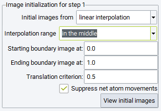
Setting the Interpolation range to in the middle, parts of the reaction path can be excluded from optimization by specifying the Starting boundary image and Ending boundary image path parameters. For example, when a reaction occurs close to a surface, but the initial or final configurations are in quite some distance from the surface, these options allow omission of the physisorption part of the reactants and products. It is noted, however, that the new boundary images are affected by linear interpolation and do not correspond to local minima. It is recommended to avoid these options by finding initial and final configurations close to the surface prior to transition state search.
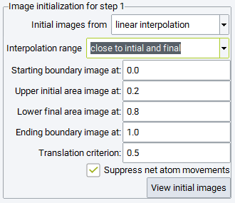
Setting the Interpolation range to close to initial and final, the interpolated images are accumulated close to the initial and final configurations. Specifically, half of the images are created between the Starting boundary image and Upper initial area image path parameters, whereas the other half is interpolated between the Lower final area image and Ending boundary image path parameters. This setting is recommended, if unphysical images would occur in the range between Upper initial area image and Lower final area image upon interpolating the full range. Since the nudged elastic band technique enforces equidistant images during optimization, the images will move into the middle range avoiding close contacts between atoms, which would occur interpolating linearly in the entire range. In order to speed up the redistribution of images, an order of magnitude larger spring constants and low precision VASP parameters are recommended. Such a simulation could be run prior to the actual Transition State Search simulation, with the sole objective to obtain physically reasonable initial images, which can be introduced into the subsequent simulation in the following way:
You can select Initial images from specified systems to define a specific pathway. Those can be obtained by the procedure as outlined above, or maybe partially based on the structures from linear interpolation.
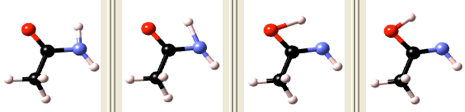
You can click on View initial images to inspect the images generated by any of the interpolation modes.
2.17.2.5. Configurations
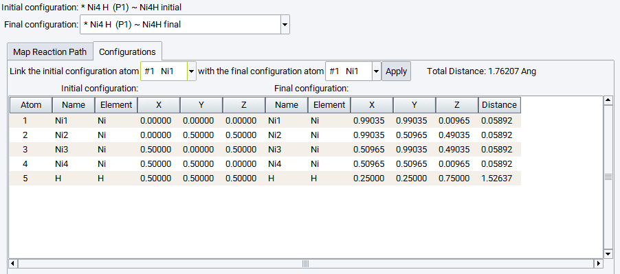
Click on the Configurations tab to inspect the matching between the individual atoms and apply corrections if needed. Each atom of the initial and final configuration needs to correspond to each other, appearing in the same line of the table. If this is not the case, the sequence of atoms of the final configuration can be modified by choosing atoms to be matched and applying the change. These modifications directly update the final configuration model beneath.
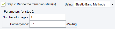
2.17.2.6. Step 2: Refine the Transition State(s) Using Elastic Band Methods
A second simulation step can be selected to refine the transition state candidate(s) obtained in the first step by two different methods. Using Elastic Band Methods performs a Climbing Image Nudged Elastic Band simulation between the images found adjacent to the transition state position in the first step with Number of images and Convergence criterion is chosen independently from those in the first simulation step. All other parameters for the elastic band method are applied as set for step 1.
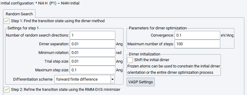
2.17.2.7. Step 2: Refine the Transition State(s) Using Dimer Method
Alternatively, the transition state candidate can be further refined Using Dimer Method, which is a minimization technique following the lowest eigenmode of the Hessian. The following parameters trigger the performance of the Dimer Method:
The Convergence criterion and the Maximum number of steps are set independently of those set in Step 1.
Dimer separation: the stepsize for numerical differentiation
Minimum rotation: the dimer is rotated only if the predicted rotation angle is greater than this value
Trial step size: the trial step size for the optimization step
Maximum step size: the trust radius (upper limit) for the optimization step
Differentiation scheme: whether to use a forward finite difference or a central finite difference formula for the numerical differentiation to compute the curvature along the dimer direction
2.17.2.8. Step 3: Refine the Transition State(s) Using the RMM-DIIS Minimizer
Check the box next to Refine the transition state(s) using RMM-DIIS minimizer to apply RMM-DIIS optimization to the approximate saddle point structure obtained by the search process specified above. The convergence radius of this method is rather small and requires an initial structure very close to the optimized transition state.
Ensure that the transition state is well approximated by the search process, e.g. based on one or more refinement steps or the climbing image procedure and sufficiently strict convergence criteria in the first step, and/or by including a second refinement step. The attempted optimization may fail, in such a case the structure of the transition state converges back towards a local minimum energy configuration. If the optimization succeeds the optimized transition state can be used for subsequent phonon calculations to derive temperature dependent thermodynamic functions.
2.17.3. Output for Reaction Path Mapping
2.17.3.1. Job.out
The detailed output file describes the method and parameters chosen for the transition state search as well as the computational parameters of the underlying Vasp calculations, followed by one or more (for refinements) tables of energies with additional notes of accepted steps and climbing of certain images summarizing the optimization process.
The results of transition state refinement Using Dimer Method in step 2 and RMM-DIIS optimization in step 3 is indicated by headers as shown below, followed by the output as obtained after a standard VASP geometry optimization. The results for transition state refinement Using Elastic Band Methods are presented like a refinement step, however, with a different number of images.
Job.out output for: C2 N O H5 (P1) ~ Lactam (Transition State Search)
Transition State Search
Status: finished
Opening the database
2.17.3.1.1. Settings for the Transition State Search Method
Nudged Elastic Band for mapping the minimum energy path between
the initial system Lactam
and the final system Lactim
with 4 intermediate images and a spring constant of 5 eV/Ang^2 and 1
refinement steps.
The image closest to a saddle point is allowed to climb up into the
saddle point if the largest force on an atom is smaller than 2.0 eV/Ang.
Double nudging is applied.
The initial images are created from linear interpolation.
In a second step, transition states are searched for all identified
saddle points by the Dimer Method.
In the last step, an optimization of transition states by the RMM-DIIS
algorithm is attempted.
Optimization parameters for the first step:

  SCF of each iteration is started from wave functions of the previous
  iteration.
  Convergence: 0.1 eV/Ang
  Number of steps: 50
  Diagonal elements of the inverse Hessian are initially set to 0.001 Ang^2/eV.
2.17.3.1.2. VASP Parameters for Energy and Force Evaluation
VASP Parameters
===============
Since no magnetic moments are in the model, this is a non-magnetic
calculation using 'normal' precision and a default planewave cutoff
energy of 400.000 eV.
The electronic iterations convergence is 5.00E-005 eV using the Normal
(blocked Davidson) algorithm and reciprocal space projection operators.

The requested k-spacing is 2 per Angstrom, which leads to a 1x1x1 mesh.

This corresponds to actual k-spacings of 0.628 x 0.628 x 0.628 per
Angstrom.
The k-mesh is forced to be centered on the gamma point and have
an odd number of points in each direction.

Using Gaussian smearing with a width of 0.2 eV.

...
2.17.3.1.3. Progress Report on Initial Elastic Band Calculation
energy of initial and final boundary images:

    neb0_image00   -52.02879
    neb0_image05   -51.51119

Iter Energy_total max grad      image01   image02   image03   image04     Climbing  Iter accepted
---- ---------------- --------- --------- --------- --------- ------------ --- ----
1    -202.6491        4.16075  -51.50119  -50.23082  -49.91524  -51.00185
2    -203.4190        3.24538  -51.57999  -50.45669  -50.16507  -51.21725        1
3    -203.9750        2.13960  -51.66990  -50.62331  -50.41716  -51.26464        2
4    -204.2142        1.67717  -51.70906  -50.70128  -50.50220  -51.30166        3
5    -204.5963        1.97452  -51.80592  -50.84563  -50.59221  -51.35256 3      4
6    -204.6202        2.05897  -51.81996  -50.85894  -50.57911  -51.36224 3      5
7    -204.4129        1.79681  -51.92725  -50.85894  -50.23027  -51.39643 3      6
8    -204.5863        1.25600  -51.92841  -50.93486  -50.31307  -51.41000 3      7
9    -204.6790        1.22024  -51.91176  -50.97526  -50.39093  -51.40108 3      8
10   -204.7024        0.76111  -51.93584  -51.00175  -50.35292  -51.41191 3      9
Iterations: 9 using 10 calls to the function
for the transition state search by the dimer method:
---------------------------------------------------
Dimer calculation for finding the transition state starting from
the initial system neb2_max1_image01_1
with an initial dimer orientation towards the system
neb1_max1_image02_1
2.17.3.1.4. Report on Transition State Refinement by the Dimer Method:
Results for the Transition State Search by the Dimer Method:
-------------------------------------------------------------
Dimer calculation for finding the transition state starting from
the initial system neb2_max1_image01_1
with an initial dimer orientation towards the system
neb1_max1_image02_1
2.17.3.1.5. Report on Transition State Optimization by the RMM-DIIS Minimizer:
Results for the Attempted Transition State Optimization:
------------------------------------------------------------
2.17.3.2. Energy Profile
Select Transition State Search >> Energy Profile to visualize results from completed transition state searches running the task Map the reaction path and find transition states.
The Energy Profile panel graphically summarizes the results of the transition state search in terms of energy profiles for each refinement step and provides access to all structures of the images as well as trajectories of the optimization process. In addition, images can be selected and removed from the graph and thereby custom energy profiles can be created for publication and presentation purposes. For the custom profiles the reaction pathway can be animated, visualizing the structural evolution during the reaction. The capabilities and functionality of the Energy Profile panel are discussed in more detail below.
In the graph pane the energy of the individual images and transition states are plotted against the reaction coordinate x, which is a measure for the progress of the reaction from the initial (x=0) to the final configuration (x=1). All energies are given with respect to the energy of the initial state. Two definitions for the reaction coordinate can be applied and are toggled by the choice Type in the Display option frame below the graph:
1. initial coordinate / energy refers to a nominal coordinate solely based on the number of intermediate images not involving a distance metric. As an example, if 3 images are specified they appear at coordinates 0.25, 0.5 and 0.75, if 4 images are specified the formal coordinates are 0.2, 0.4, 0.6, and 0.8. The coordinates for images of refinements are defined in the same manner as subdivisions. This type of reaction coordinate indicates how images are set up initially and does not depend on the structural result of the optimization.
2. optimized coordinate / energy involves a distance metric and thereby takes into account the structural evolution during the optimization. The distance between two adjacent images is calculated as the norm of the generalized distance vectors involving differences in coordinates for all pairs of matched atoms in both images. The reaction coordinate of image k is defined as the fraction of the sum of distances between initial configuration and image k to the total sum of distances between all n images of the chain.
For refinements the reaction coordinates of boundary images are kept at their values and the intermediate images of the refinement are calculated by the above definition between these values.
For transition states the initial coordinate is defined as shown above whereas the optimized coordinate is defined as the relative distance between transition the state and initial configuration to the overall distance between initial and final configuration
Differences in energy can be measured by dragging the black measurement lines vertically, for instance to measure the activation energy or the reaction energy. The vertical black bar indicates the energy difference and can be dragged horizontally to a convenient position in the graph. The display of the measurement lines can be switched off by clicking the Measuring lines checkbox in the Display options frame.
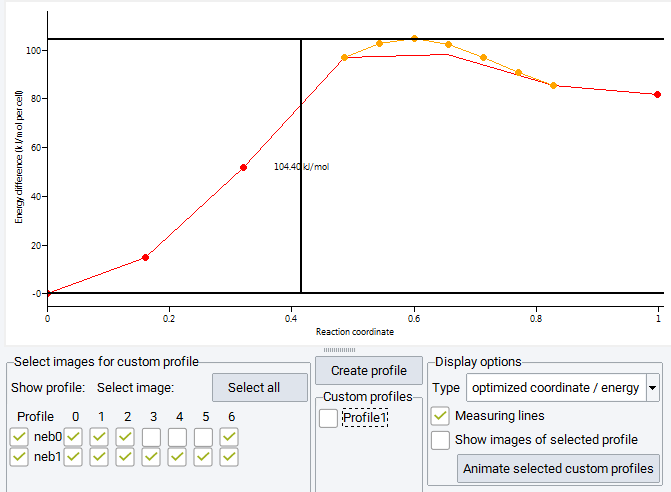
In the barrier shown above the red markers indicate image energies of the initial nudged elastic band run. Results from a further refinement step are shown in orange, where for the second step 5 images are placed between previous images with the highest energy; that is between images 3-4-5 of the initial chain to capture the path through the transition state in more detail. In the frame titled Select images for custom profiles, display of the curves connecting images is toggled by the checkboxes named neb0 and neb1 for the initial nudged elastic band run and the refinement step. The images to be displayed as markers are selected from the table of checkboxes to the right. You notice, that some images are not selected, as the image 3 of the initial chain becomes image 0 of the refinement step.
The selection of images from the table of checkboxes does not only toggle the display of markers but allows for the creation of custom energy profiles. Images apparently pulled off the minimum energy path, e.g. by spring forces acting across large distances, can be removed from the graph and for a subset of images a new energy profile is created by pushing the Create profile button above the center Custom profiles frame. This adds a custom profile colored in blue connecting only the selected images and a button Profile 1 for toggling its display is created in the Custom profiles frame. Multiple custom profiles can be created bringing up further buttons Profile 2 etc. All colored markers can be displayed by pushing the Select all button, or can be removed with the Unselect all button (showing up only if all images are selected). In order to recover the information, which images are used to create a custom profile, check on the Show images of selected profile which displays these images as blue markers.
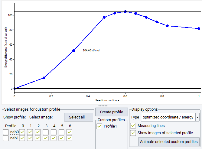
The structural evolution along the reaction pathway can be visualized as trajectory animation. Over-barrier animation is only accessible for selected (i.e. displayed) blue custom profiles and can be launched by pushing the Animate selected custom profiles button at the bottom of the Display options frame.
Transition states are indicated in the energy profile panel by pink triangles for the initial guess and by blue diamonds for their position after attempting optimization by RMM-DIIS in step 3. The results of Dimer Method optimization of step 2 are displayed as a pink plus for the initial structure and as a blue rectangle for the optimized transition state structure. The buttons named for instance TS1 initial and TS1 final allow toggling display as well as to select them for being included in custom profiles. These markers are not shown in the figures, because only Step 1 was performed for these sample calculations.
Structure information and collected VASP output for each image and refinement step are stored on the JobServer. The optimized results are contained in the main job directory and the structural optimization history can be deduced from trajectory files. VASP output for all iterations for each image is stored in the iterations subfolder. You can use optimized images as a starting point for further refinement.
Move the cursor over an image marker in the energy profile close enough such that it becomes highlighted by a green rectangle. A right-click then provides additional items for the context menu.
View Image: displays the selected image as a MedeA structure in the framework viewer
If the selected Image is a transition state, there are two options:
View Transition State (initial) and View Transition State (final) to display the structure of the transition state before and after RMM-DIIS optimization.
Animate Trajectory: opens a window and displays the trajectory of the selected image showing the structural evolution during the optimization process. The animation can be stopped at any frame and the current structure can be created by Edit >> Duplicate. This provides access to any structure of any image during optimization.
2.17.4. Find Transition State in a Direction
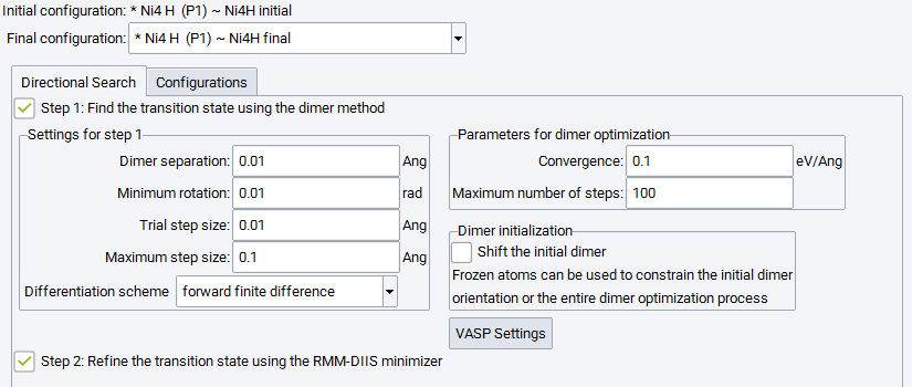
The menu item Find transition state in a direction raises the below panel to configure transition state search and optimization starting from the initial state in a direction towards another state - which doesn’t need to be a final state of a reaction - by means of the Dimer Method. The parameters triggering the performance of the Dimer Method are identical to those described in section2.vii, and also their values are identical. Running Step 1 is mandatory and cannot be deselected.
The subpanel for Dimer initialization provides two options. If the initial state is a local minimum, the Dimer Method would not be able to move towards a transition state and the optimization would finish after one step. In order to start the optimization process, Shift the initial dimer shifts the dimer towards the final configuration and enables the optimization process to start.
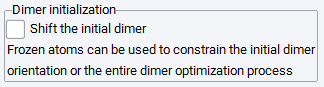
Furthermore, it might be beneficial to exclude certain degrees of freedom from the dimer initialization, which can be achieved by freezing atoms of the initial configuration. If this is the case, the Dimer initialization subpanel allows you to either take into account these constraints for the initial dimer orientation only or to keep these atoms fixed for the entire dimer optimization.
Check the box next to Refine the transition state using RMM-DIIS minimizer to apply RMM-DIIS optimization to the approximate saddle point structure obtained by the Dimer Method search.
The Configuration Tab is identical to that of the other computational tasks and is described in section 2.v.
2.17.5. Find Transition States in Random Directions
The menu item Find transition states in random directions brings up a panel to configure transition state search and optimization in a number of different randomly chosen directions by means of the Dimer Method. The number of directions can be specified by Number of random search directions.
For random search directions it is particularly important to restrict the possible search direction by means of chemical intuition. It is recommended to freeze all those atoms that are not expected to be involved in the reaction, and to keep them fixed at least for the initial dimer orientation only.
Check the box next to Refine the transition state using RMM-DIIS minimizer to apply RMM-DIIS optimization to each of the approximate saddle point structures obtained by the dimer search of the first step.
| download: | pdf |
|---|